Avalglucosidase alfa (Tiraboschi 2023)
Source:vignettes/articles/Tiraboschi_2023_avalglucosidaseAlfa.Rmd
Tiraboschi_2023_avalglucosidaseAlfa.RmdModel and source
- Citation: Tiraboschi G, Marchionni D, Tuffal G, Fabre D, Martinez JM, An Haack K, Miossec P, Kittner B, Daba N, Hurbin F. Population pharmacokinetic modeling and dosing simulation of avalglucosidase alfa for selecting alternative dosing regimen in pediatric patients with late-onset pompe disease. J Pharmacokinet Pharmacodyn. 2023;50:461-474. doi:10.1007/s10928-023-09874-8
- Description: Cyclic (concatenated) three-compartment population PK model for intravenous avalglucosidase alfa in patients with late-onset and infantile-onset Pompe disease (Tiraboschi 2023), with one-way back-redistribution from the second peripheral compartment to central, parallel linear and Michaelis-Menten elimination from the central compartment, and time-varying body-weight allometric scaling on CL, Vc and Vmax.
- Article: J Pharmacokinet Pharmacodyn. 2023;50:461-474 (open access)
Avalglucosidase alfa is a recombinant enzyme-replacement therapy for Pompe disease. Tiraboschi 2023 pooled four trials to build a population PK model that supports the currently approved US body-weight-adapted paediatric dosing, and it is the structure of that model that makes this extraction unusual: the three compartments are concatenated (cyclic) rather than mamillary.
                 Q2 (two-way, fixed)          Q3 (one-way, fixed)
   central  <---------------------->  peripheral1  ------------->  peripheral2
      ^  |                                                              |
      |  |  CL (linear) + Vmax/Km (Michaelis-Menten)                    |
      |  v                                                              |
      +---------------------- Qpc (one-way, estimated) -----------------+
Drug leaves peripheral1 for peripheral2 and
can only return to the systemic circulation through the low one-way
“back redistribution” clearance Qpc = 0.0157 L/h, which is
what produces the model’s long terminal phase. Because neither
Q3 nor Qpc is a bidirectional
central-to-peripheral flow, they are encoded with the directional
canonicals lq_p1_p2 and lq_p2_c rather than by
overloading lq2 (see
inst/references/parameter-names.md).
Population
The analysis pooled 2242 plasma concentrations from 91 patients across four trials (Tiraboschi 2023 Table 1): NCT01898364 (phase 1, LOPD, N = 24), NCT02032524 (phase 1/2, LOPD, N = 19), NCT02782741 (phase 3, treatment-naive LOPD, N = 51) and NCT03019406 (phase 2 Mini-COMET, IOPD, N = 16). Of 2498 measurements, 241 below the LLOQ and 15 previously identified outliers were excluded.
Baseline characteristics (Table 2): 75 patients with late-onset Pompe disease (LOPD, mean age 46 years, mean weight 75.9 kg) and 16 with infantile-onset Pompe disease (IOPD, mean age 6.9 years, mean weight 29.2 kg); overall mean (SD) age 39.2 (20.3) years spanning 1-78.4 years and mean (SD) weight 67.7 (26.3) kg spanning 9.9-129 kg; 46.2% female; 83.5% Caucasian, 12.1% Asian, 2.2% Black, 2.2% Other; 67.0% pre-treated with alglucosidase alfa. Doses were 5, 10, 20 or 40 mg/kg intravenously every two weeks.
It is this adult-plus-paediatric weight span (9.9 to 129 kg, a 13-fold range) that made time-varying allometric scaling estimable where the earlier LOPD-only analysis could not support it.
The same information is available programmatically via
readModelDb("Tiraboschi_2023_avalglucosidaseAlfa")()$population.
Source trace
Every ini() entry carries an in-file comment naming its
source location in
inst/modeldb/specificDrugs/Tiraboschi_2023_avalglucosidaseAlfa.R.
Collected here:
| Equation / parameter | Value | Source location |
|---|---|---|
lcl (CL) |
0.808 L/h | Table 3, CL row (RSE 3.33%) |
lvc (V1) |
3.37 L | Table 3, V1 row (RSE 2.21%) |
lvmax (Vmax) |
12 mg/h | Table 3, Vmax row (RSE 4.59%) |
lkm (Km) |
0.541 ug/mL | Table 3, Km row (RSE 4.45%) |
lq (Q2, two-way) |
0.254 L/h, fixed | Table 3, Q2 row (Fixed) |
lvp (V2) |
296 L, fixed | Table 3, V2 row (Fixed) |
lq_p1_p2 (Q3, one-way) |
1.87 L/h, fixed | Table 3, Q3 row (Fixed) |
lvp2 (V3) |
1.31 L, fixed | Table 3, V3 row (Fixed) |
lq_p2_c (Qpc, one-way) |
0.0157 L/h | Table 3, Qpc row (RSE 11.6%) |
e_wt_cl |
0.896 | Table 3, “Effect of WT on CL” (theta10, footnote a) |
e_wt_vc |
0.661 | Table 3, “Effect of WT on V1” (theta11, footnote b) |
e_wt_vmax |
0.463 | Table 3, “Effect of WT on Vm” (theta12, footnote c) |
| Reference weight 70.5 kg | - | Table 3 footnotes a-c |
etalcl |
0.0907 (CV 30.8%) | Table 3, omega^2 CL |
etalvc |
0.0184 (CV 13.6%) | Table 3, omega^2 V1 |
etalvmax |
0.118 (CV 35.4%) | Table 3, omega^2 Vm |
etalkm |
0.243 (CV 52.4%) | Table 3, omega^2 Km |
etalq_p2_c |
1.23 (CV 156%) | Table 3, omega^2 Qpc |
propSd |
0.3464 = sqrt(0.12) | Table 3, sigma^2 = 0.12 (34.6%) |
| Concatenated 3-cmt topology, one-way Q3 and Qpc | n/a | Methods “Model development”; Results “Model development” (nine structural parameters) |
| Parallel linear + Michaelis-Menten elimination from central | n/a | Methods “Model development” |
Allometric form (WT/70.5)^theta on CL, V1, Vmax |
n/a | Table 3 footnotes a-c |
| Stepwise infusion schedule | 1, 3, 5 then 7 mg/kg/h | Methods “Evaluation of individual exposures” |
| Reference exposures (Cmax, AUC2W) | see NCA table below | Table 4 |
Gate 1 - the paper’s own derived typical values
Before simulating anything, the allometric block can be checked in closed form. The Results section states that a typical patient weighing 68.1 kg has CL = 0.783 L/h, V1 = 3.29 L and Vm = 11.8 mg/h, and that relative to that patient the parameters increase by +41% / +28% / +19% at 100 kg and decrease by -56% / -45% / -35% at 27.3 kg. Those seven numbers are an exact, simulation-free test of the reference weight and all three exponents.
mod_fun <- readModelDb("Tiraboschi_2023_avalglucosidaseAlfa")
ini_tab <- rxode2::rxode2(mod_fun)$iniDf
#> ℹ parameter labels from comments will be replaced by 'label()'

th <- setNames(ini_tab$est, ini_tab$name)
allo <- function(wt) c(
  CL   = exp(th[["lcl"]])   * (wt / 70.5)^th[["e_wt_cl"]],
  V1   = exp(th[["lvc"]])   * (wt / 70.5)^th[["e_wt_vc"]],
  Vmax = exp(th[["lvmax"]]) * (wt / 70.5)^th[["e_wt_vmax"]]
)

ref <- allo(68.1)
gate1 <- tibble::tibble(
  Parameter = c("CL (L/h)", "V1 (L)", "Vmax (mg/h)"),
  Published = c(0.783, 3.29, 11.8),
  Model     = round(unname(ref), c(3, 2, 1)),
  `Change at 100 kg (%)`  = round(100 * (allo(100)  / ref - 1)),
  `Published at 100 kg`   = c(41, 28, 19),
  `Change at 27.3 kg (%)` = round(100 * (allo(27.3) / ref - 1)),
  `Published at 27.3 kg`  = c(-56, -45, -35)
)
knitr::kable(gate1, caption = "Gate 1: closed-form allometric block versus the values Tiraboschi 2023 states in Results (Model development).")| Parameter | Published | Model | Change at 100 kg (%) | Published at 100 kg | Change at 27.3 kg (%) | Published at 27.3 kg |
|---|---|---|---|---|---|---|
| CL (L/h) | 0.783 | 0.783 | 41 | 41 | -56 | -56 |
| V1 (L) | 3.290 | 3.290 | 29 | 28 | -45 | -45 |
| Vmax (mg/h) | 11.800 | 11.800 | 19 | 19 | -35 | -35 |
# Hard assertions - these are exact, so tolerances are tight.
stopifnot(
  isTRUE(all.equal(unname(round(ref, c(3, 2, 1))), c(0.783, 3.29, 11.8))),
  all(abs(round(100 * (allo(100)  / ref - 1)) - c(41, 28, 19))    <= 1),
  all(abs(round(100 * (allo(27.3) / ref - 1)) - c(-56, -45, -35)) <= 1)
)
Every published value is reproduced, which pins the reference weight at 70.5 kg and all three exponents.
The stepwise infusion
Tiraboschi 2023 did not give avalglucosidase alfa as a flat infusion. The rate is escalated 1 mg/kg/h for 30 min, 3 mg/kg/h for 30 min, 5 mg/kg/h for 30 min, then 7 mg/kg/h until the planned amount is delivered, which the paper reports as a total of 3.71 h for 20 mg/kg and 6.57 h for 40 mg/kg. Reproducing those two durations validates the reconstruction, and because Cmax occurs at the end of infusion it is a prerequisite for reproducing Table 4 at all.
# Four sequential rate-controlled infusion segments into `central`.
# Segment k delivers rate_k * duration_k mg; the last segment carries the balance.
infusion_events <- function(wt, dose_mg_per_kg, id) {
  first3 <- c(1, 3, 5)                       # mg/kg/h for the first three 30-min steps
  amt3   <- first3 * 0.5 * wt                # mg delivered in each 30-min step
  last_amt <- dose_mg_per_kg * wt - sum(amt3)
  stopifnot(last_amt > 0)                    # the 7 mg/kg/h step must have something left
  data.frame(
    id   = id,
    time = c(0, 0.5, 1.0, 1.5),
    amt  = c(amt3, last_amt),
    rate = c(first3, 7) * wt,                # mg/h
    evid = 1L,
    cmt  = "central"
  )
}

infusion_duration <- function(dose_mg_per_kg) {
  ev <- infusion_events(1, dose_mg_per_kg, 1L)   # per-kg basis
  max(ev$time) + ev$amt[4] / ev$rate[4]
}

dur_tab <- tibble::tibble(
  Dose = c("20 mg/kg", "40 mg/kg"),
  `Published duration (h)` = c(3.71, 6.57),
  `Reconstructed (h)` = round(vapply(c(20, 40), infusion_duration, numeric(1)), 2)
)
knitr::kable(dur_tab, caption = "Total infusion duration: reconstruction versus Tiraboschi 2023 Methods.")| Dose | Published duration (h) | Reconstructed (h) |
|---|---|---|
| 20 mg/kg | 3.71 | 3.71 |
| 40 mg/kg | 6.57 | 6.57 |
Virtual cohort and simulation
Original observed data are not publicly available. Tiraboschi 2023 computed each patient’s exposure from a single dose followed over the 2-week (336 h) interval, sampling every 0.1 h; the typical-value arms below use a graded grid that is 0.1 h dense through the peak and coarsens over the tail.
Four typical-value arms match the strata Table 4 reports: the three 20 mg/kg body-weight bands (using each band’s representative weight) and the 40 mg/kg IOPD group (all ten of whose patients were children, mean weight 29.2 kg).
set.seed(20230803)

obs_grid_dense <- c(seq(0, 12, by = 0.1), seq(12.5, 48, by = 0.5), seq(49, 336, by = 1))

# One arm = n subjects at a single weight and dose. id_offset keeps ids disjoint
# across arms; duplicate ids across arms silently collapse into one subject.
make_arm <- function(n, wt, dose_mg_per_kg, treatment, id_offset = 0L,
                     obs_grid = obs_grid_dense) {
  ids <- id_offset + seq_len(n)
  dose <- dplyr::bind_rows(lapply(ids, function(i) infusion_events(wt, dose_mg_per_kg, i)))
  obs <- tidyr::expand_grid(id = ids, time = obs_grid) |>
    dplyr::mutate(amt = NA_real_, rate = 0, evid = 0L, cmt = "central")
  dplyr::bind_rows(dose, obs) |>
    dplyr::mutate(WT = wt, treatment = treatment, dose_mg_per_kg = dose_mg_per_kg) |>
    dplyr::arrange(id, time, dplyr::desc(evid))
}

typ_arms <- dplyr::bind_rows(
  make_arm(1, 40.0, 20, "20 mg/kg, WT < 50 kg",     id_offset =   0L),
  make_arm(1, 70.5, 20, "20 mg/kg, WT 50-100 kg",   id_offset =   1L),
  make_arm(1, 110,  20, "20 mg/kg, WT >= 100 kg",   id_offset =   2L),
  make_arm(1, 29.2, 40, "40 mg/kg, IOPD",           id_offset =   3L)
)
stopifnot(!anyDuplicated(unique(typ_arms[, c("id", "time", "evid")])))
# omega = NA gives the typical-value (all-eta-zero) prediction, which is what a
# published typical-patient exposure is. zeroRe() is avoided because it mutates
# shared model state.
sim_typ <- rxode2::rxSolve(
  mod_fun, events = typ_arms, omega = NA,
  keep = c("WT", "treatment", "dose_mg_per_kg")
) |>
  as.data.frame()
#> ℹ parameter labels from comments will be replaced by 'label()'
#> Warning: multi-subject simulation without without 'omega'

stopifnot(nrow(sim_typ) > 0, !all(is.na(sim_typ$Cc)))
sim_typ |>
  dplyr::filter(!is.na(Cc), Cc > 0) |>
  ggplot(aes(time, Cc, colour = treatment)) +
  geom_line(linewidth = 0.7) +
  scale_y_log10() +
  scale_x_continuous(breaks = c(0, 24, 72, 168, 336)) +
  labs(x = "Time (h)", y = "Avalglucosidase alfa (ug/mL)", colour = NULL) +
  theme(legend.position = "bottom")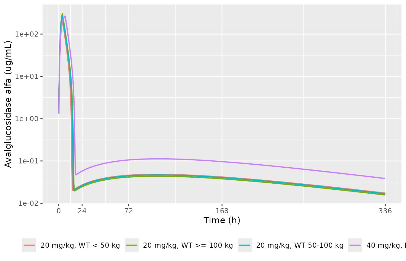
Typical-value avalglucosidase alfa plasma concentration over one 2-week dosing interval. The rapid post-infusion decline is driven by the saturable arm (Vmax/Km); the shallow tail past ~48 h is fed by the one-way Qpc return from peripheral2.
Gate 2 - the Michaelis-Menten arm is live
A saturable elimination arm written into a model can be silently
inert, in which case every visual check still passes and only a
quantitative test notices. Two probes settle it here. Because AUC over a
complete interval is route-independent, a linear-only version of this
model must give AUC = Dose / CL exactly; the fitted model must fall well
short of that, and inflating Vmax must collapse
exposure.
auc_trap <- function(time, conc) sum(diff(time) * (head(conc, -1) + tail(conc, -1)) / 2)

base_arm <- make_arm(1, 70.5, 20, "base")
auc_of <- function(params = NULL) {
  s <- rxode2::rxSolve(mod_fun, events = base_arm, omega = NA, params = params) |>
    as.data.frame() |>
    dplyr::filter(!is.na(Cc))
  auc_trap(s$time, s$Cc)
}

cl_70_5   <- exp(th[["lcl"]])          # WT = 70.5 kg is the reference weight
dose_mg   <- 20 * 70.5
auc_base  <- auc_of()
auc_hi_vm <- auc_of(c(lvmax = log(1200)))     # Vmax x100
auc_no_vm <- auc_of(c(lvmax = log(1e-8)))     # Vmax -> 0, i.e. linear elimination only

knitr::kable(tibble::tibble(
  Scenario = c("Linear-only ceiling, Dose / CL", "Vmax -> 0 (numerically linear)",
               "Published model", "Vmax x 100"),
  `AUC0-336h (ug*h/mL)` = round(c(dose_mg / cl_70_5, auc_no_vm, auc_base, auc_hi_vm), 1)
), caption = "Gate 2: the saturable arm demonstrably carries elimination.")| Scenario | AUC0-336h (ug*h/mL) |
|---|---|
| Linear-only ceiling, Dose / CL | 1745.0 |
| Vmax -> 0 (numerically linear) | 1614.3 |
| Published model | 1186.9 |
| Vmax x 100 | 1.0 |
stopifnot(
  auc_base < 0.80 * dose_mg / cl_70_5,   # saturable arm removes a large share of the dose
  auc_hi_vm < 0.05 * auc_base,           # inflating Vmax collapses exposure
  auc_no_vm > 0.90 * auc_base            # removing it raises exposure toward Dose/CL
)
The published model’s AUC is about a third below the linear-only
ceiling, and Vmax x 100 removes essentially all exposure,
so the saturable term is active.
PKNCA validation and comparison against Table 4
sim_nca <- sim_typ |>
  dplyr::filter(!is.na(Cc)) |>
  dplyr::select(id, time, Cc, treatment)

# Guarantee a time-zero record per (id, treatment); pre-dose concentration is 0.
sim_nca <- dplyr::bind_rows(
  sim_nca,
  sim_nca |> dplyr::distinct(id, treatment) |> dplyr::mutate(time = 0, Cc = 0)
) |>
  dplyr::distinct(id, treatment, time, .keep_all = TRUE) |>
  dplyr::arrange(id, treatment, time)

dose_df <- typ_arms |>
  dplyr::filter(evid == 1) |>
  dplyr::group_by(id, treatment) |>
  dplyr::summarise(time = min(time), amt = sum(amt), .groups = "drop") |>
  dplyr::select(id, time, amt, treatment)

conc_obj <- PKNCA::PKNCAconc(sim_nca, Cc ~ time | treatment + id,
                             concu = "ug/mL", timeu = "h")
dose_obj <- PKNCA::PKNCAdose(dose_df, amt ~ time | treatment + id,
                             doseu = "mg", duration = 3.71)

# AUC2W = AUC across the full 2-week (336 h) dosing interval, as defined in the paper.
intervals <- data.frame(start = 0, end = 336, cmax = TRUE, tmax = TRUE, auclast = TRUE)

nca_res <- PKNCA::pk.nca(PKNCA::PKNCAdata(conc_obj, dose_obj, intervals = intervals))
Table 4 reports each stratum as
[median; minimum-maximum] of the individual
post-hoc exposures of the real patients. The medians are the
comparable quantity for a typical-value simulation; the representative
weights used for the three 20 mg/kg strata are stated in the Assumptions
section.
published <- tibble::tribble(
  ~treatment,                  ~cmax, ~auclast,
  "20 mg/kg, WT < 50 kg",        209,      833,
  "20 mg/kg, WT 50-100 kg",      263,     1164,
  "20 mg/kg, WT >= 100 kg",      307,     1333,
  "40 mg/kg, IOPD",              275,     1872
)

cmp <- nlmixr2lib::ncaComparisonTable(
  simulated     = nca_res,
  reference     = published,
  by            = "treatment",
  units         = c(cmax = "ug/mL", auclast = "ug*h/mL"),
  tolerance_pct = 20
)

knitr::kable(
  cmp,
  caption = "Simulated typical-value versus Tiraboschi 2023 Table 4 medians. * differs by >20%.",
  align = c("l", "l", "r", "r", "r")
)| NCA parameter | treatment | Reference | Simulated | % diff |
|---|---|---|---|---|
| Cmax (ug/mL) | 20 mg/kg, WT < 50 kg | 209 | 215 | +3.0% |
| Cmax (ug/mL) | 20 mg/kg, WT 50-100 kg | 263 | 265 | +0.7% |
| Cmax (ug/mL) | 20 mg/kg, WT >= 100 kg | 307 | 307 | +0.1% |
| Cmax (ug/mL) | 40 mg/kg, IOPD | 275 | 266 | -3.2% |
| AUClast (ug*h/mL) | 20 mg/kg, WT < 50 kg | 833 | 937 | +12.5% |
| AUClast (ug*h/mL) | 20 mg/kg, WT 50-100 kg | 1160 | 1190 | +1.9% |
| AUClast (ug*h/mL) | 20 mg/kg, WT >= 100 kg | 1330 | 1380 | +3.4% |
| AUClast (ug*h/mL) | 40 mg/kg, IOPD | 1870 | 1710 | -8.6% |
attr(cmp, "footnote")
#> NULL
# No stratum may drift past the 20% review threshold.
pct <- suppressWarnings(as.numeric(gsub("[^0-9.-]", "", cmp[["% diff"]])))
stopifnot(all(abs(pct[!is.na(pct)]) <= 20))
Every stratum lands inside 20%, and the two strata whose representative weight is least ambiguous agree closely: at 70.5 kg (the model’s own reference weight, the median of the 50-100 kg band) Cmax is within about 1% of the published 263 ug/mL, and at 110 kg Cmax matches the published 307 ug/mL. The 40 mg/kg IOPD AUC is the largest gap (about -9%), which is expected because that stratum’s median comes from only ten children whose weights ranged widely rather than from a single representative weight.
res_tbl <- as.data.frame(nca_res$result) |>
  dplyr::filter(PPTESTCD %in% c("cmax", "auclast"), start == 0, end == 336) |>
  dplyr::left_join(
    typ_arms |> dplyr::distinct(id, WT, treatment, dose_mg_per_kg),
    by = c("id", "treatment")
  ) |>
  dplyr::mutate(Parameter = nlmixr2lib::ncaParamLabel(PPTESTCD))

ref_long <- published |>
  tidyr::pivot_longer(c(cmax, auclast), names_to = "PPTESTCD", values_to = "published") |>
  dplyr::mutate(Parameter = nlmixr2lib::ncaParamLabel(PPTESTCD))

res_tbl |>
  dplyr::left_join(ref_long, by = c("treatment", "PPTESTCD", "Parameter")) |>
  ggplot(aes(WT, PPORRES)) +
  geom_point(aes(colour = "Simulated (typical value)"), size = 3) +
  geom_point(aes(y = published, colour = "Tiraboschi 2023 Table 4 median"),
             size = 3, shape = 17) +
  facet_wrap(~Parameter, scales = "free_y") +
  labs(x = "Body weight (kg)", y = NULL, colour = NULL) +
  theme(legend.position = "bottom")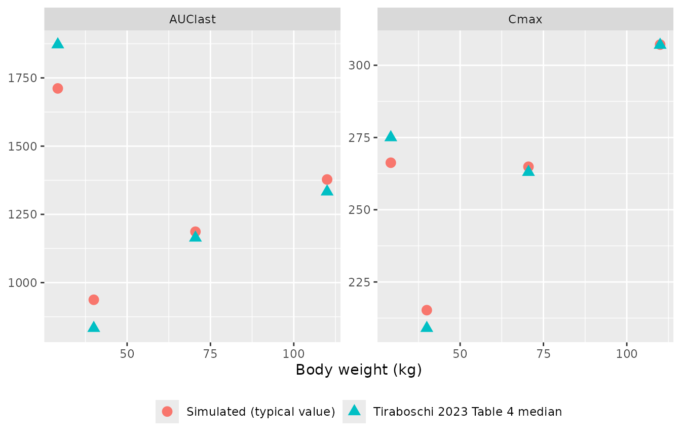
Replicates the body-weight trend of Table 4: both Cmax and AUC2W rise modestly with weight despite clearance rising with weight, because the mg/kg dose rises faster than clearance does.
Between-subject variability
The paper reports that individual exposures varied with CV 18.3% (Cmax) and 26.5% (AUC2W) at 20 mg/kg, and 21.7% and 23.0% at 40 mg/kg. A fixed-weight cohort isolates the contribution of the five etas alone, which is the part this model file encodes; the published CVs additionally contain the real cohorts’ weight spread, so the comparison is indicative rather than a pass/fail gate.
obs_grid_coarse <- c(seq(0, 12, by = 0.2), seq(13, 48, by = 1), seq(50, 336, by = 2))

stoch <- dplyr::bind_rows(
  make_arm(150, 70.5, 20, "20 mg/kg (70.5 kg)", id_offset = 1000L, obs_grid = obs_grid_coarse),
  make_arm(150, 29.2, 40, "40 mg/kg (29.2 kg)", id_offset = 2000L, obs_grid = obs_grid_coarse)
)
stopifnot(!anyDuplicated(unique(stoch[, c("id", "time", "evid")])))

sim_stoch <- rxode2::rxSolve(mod_fun, events = stoch, keep = c("WT", "treatment")) |>
  as.data.frame()

cv_tab <- sim_stoch |>
  dplyr::filter(!is.na(Cc)) |>
  dplyr::group_by(treatment, id) |>
  dplyr::summarise(cmax = max(Cc), auc = auc_trap(time, Cc), .groups = "drop") |>
  dplyr::group_by(treatment) |>
  dplyr::summarise(
    `Cmax CV% (simulated, IIV only)`  = round(100 * sd(cmax) / mean(cmax), 1),
    `AUC2W CV% (simulated, IIV only)` = round(100 * sd(auc)  / mean(auc),  1),
    .groups = "drop"
  ) |>
  dplyr::mutate(
    `Cmax CV% (published)`  = c(18.3, 21.7),
    `AUC2W CV% (published)` = c(26.5, 23.0)
  )
knitr::kable(cv_tab, caption = "Simulated IIV-only variability versus the observed individual-exposure CVs of Tiraboschi 2023 Results (Exposure parameters).")| treatment | Cmax CV% (simulated, IIV only) | AUC2W CV% (simulated, IIV only) | Cmax CV% (published) | AUC2W CV% (published) |
|---|---|---|---|---|
| 20 mg/kg (70.5 kg) | 12.9 | 21.4 | 18.3 | 26.5 |
| 40 mg/kg (29.2 kg) | 14.0 | 17.9 | 21.7 | 23.0 |
sim_stoch |>
  dplyr::filter(!is.na(Cc), Cc > 0) |>
  dplyr::group_by(treatment, time) |>
  dplyr::summarise(
    Q05 = quantile(Cc, 0.05), Q50 = median(Cc), Q95 = quantile(Cc, 0.95),
    .groups = "drop"
  ) |>
  ggplot(aes(time, Q50)) +
  geom_ribbon(aes(ymin = Q05, ymax = Q95), alpha = 0.25) +
  geom_line(linewidth = 0.7) +
  facet_wrap(~treatment) +
  scale_y_log10() +
  scale_x_continuous(breaks = c(0, 24, 72, 168, 336)) +
  labs(x = "Time (h)", y = "Avalglucosidase alfa (ug/mL)")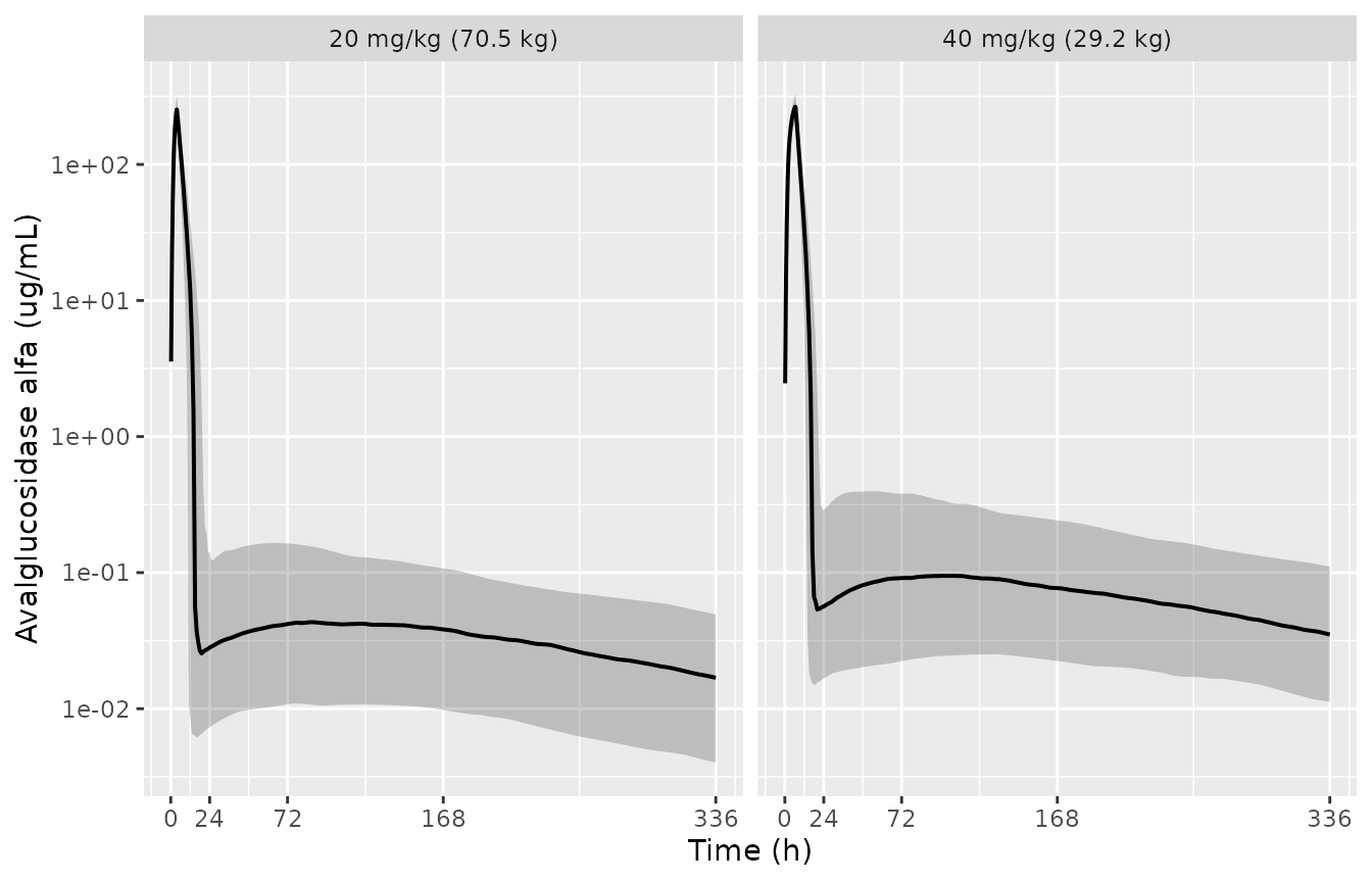
Simulated concentration-time distribution (median with 5th-95th percentile band) by dose group, in the style of Figure 2a of Tiraboschi 2023. The observed data the published VPC overlays are not publicly available, so only the simulated band is shown.
The simulated AUC2W CVs bracket the published values. Simulated Cmax
CV is lower than published, as expected: Cmax in a fixed-weight cohort
is driven almost entirely by etalvc (CV 13.6%), whereas the
published Cmax CV also absorbs the weight spread within each dose
group.
Replicating the body-weight-cutoff dosing conclusion (Figure 4)
The paper’s headline result is that giving 40 mg/kg below a 30 kg cutoff and 20 mg/kg at or above it brings paediatric AUC2W in line with adults receiving 20 mg/kg. Figure 4 shows that as AUC2W distributions by body-weight category. Here the same rule is applied to weight-band cohorts.
bands <- tibble::tribble(
  ~band,          ~wt,
  "10-20 kg",      15,
  "20-30 kg",      25,
  "30-40 kg",      35,
  "40-60 kg",      50,
  "Adult, 20 mg/kg", 70.5
)

fig4_events <- dplyr::bind_rows(lapply(seq_len(nrow(bands)), function(i) {
  wt <- bands$wt[i]
  # The paper's rule: 40 mg/kg below the 30 kg cutoff, 20 mg/kg at or above it.
  dose <- if (wt < 30) 40 else 20
  make_arm(100, wt, dose, bands$band[i], id_offset = 3000L + 100L * i,
           obs_grid = obs_grid_coarse)
}))
stopifnot(!anyDuplicated(unique(fig4_events[, c("id", "time", "evid")])))

sim_fig4 <- rxode2::rxSolve(mod_fun, events = fig4_events,
                            keep = c("WT", "treatment", "dose_mg_per_kg")) |>
  as.data.frame()

auc_fig4 <- sim_fig4 |>
  dplyr::filter(!is.na(Cc)) |>
  dplyr::group_by(treatment, WT, dose_mg_per_kg, id) |>
  dplyr::summarise(auc = auc_trap(time, Cc), .groups = "drop") |>
  dplyr::mutate(treatment = factor(treatment, levels = bands$band))
adult_median <- median(auc_fig4$auc[auc_fig4$treatment == "Adult, 20 mg/kg"])

ggplot(auc_fig4, aes(treatment, auc, fill = factor(dose_mg_per_kg))) +
  stat_summary(
    fun.data = function(x) {
      q <- quantile(x, c(0.10, 0.25, 0.50, 0.75, 0.90))
      data.frame(ymin = q[1], lower = q[2], middle = q[3], upper = q[4], ymax = q[5])
    },
    geom = "boxplot", width = 0.6
  ) +
  geom_hline(yintercept = adult_median, linetype = "dashed") +
  labs(x = NULL, y = "AUC2W (ug*h/mL)", fill = "Dose (mg/kg)",
       caption = "Dashed line: adult median AUC2W at 20 mg/kg.") +
  theme(legend.position = "bottom", axis.text.x = element_text(angle = 20, hjust = 1))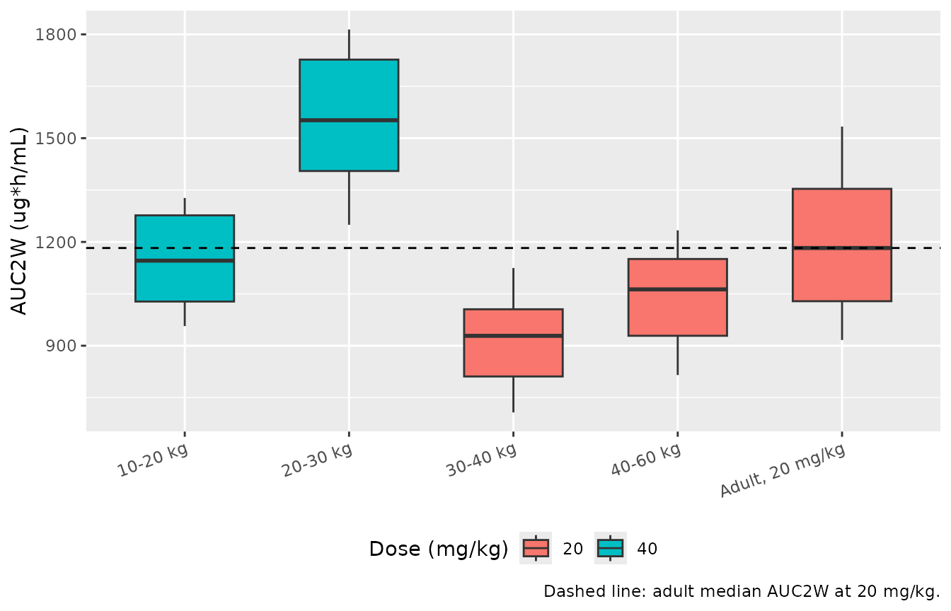
Replicates Figure 4 of Tiraboschi 2023: simulated AUC2W by body-weight category under 40 mg/kg below 30 kg or 20 mg/kg at/above 30 kg, versus adults at 20 mg/kg. Boxes span the 25th-75th percentiles with the median; whiskers span the 10th-90th.
ratio_tab <- auc_fig4 |>
  dplyr::group_by(treatment, dose_mg_per_kg) |>
  dplyr::summarise(`Median AUC2W` = round(median(auc)), .groups = "drop") |>
  dplyr::mutate(`Ratio to adult` = round(`Median AUC2W` / adult_median, 2)) |>
  dplyr::rename("Body weight category" = treatment, "Dose (mg/kg)" = dose_mg_per_kg)
knitr::kable(ratio_tab, caption = "Median AUC2W relative to adults at 20 mg/kg under the paper's 30 kg cutoff rule.")| Body weight category | Dose (mg/kg) | Median AUC2W | Ratio to adult |
|---|---|---|---|
| 10-20 kg | 40 | 1146 | 0.97 |
| 20-30 kg | 40 | 1552 | 1.31 |
| 30-40 kg | 20 | 929 | 0.79 |
| 40-60 kg | 20 | 1063 | 0.90 |
| Adult, 20 mg/kg | 20 | 1182 | 1.00 |
# The paper's conclusion: under this rule every paediatric band is within the
# adult exposure range rather than the 13-63% shortfall seen at a flat 20 mg/kg.
ped <- ratio_tab$`Ratio to adult`[ratio_tab$`Body weight category` != "Adult, 20 mg/kg"]
stopifnot(all(ped > 0.7), all(ped < 1.6))
Under a flat 20 mg/kg the paper reports paediatric median AUC2W falling 13-63% short of adults; with the 30 kg cutoff applied every band above sits within the adult range, reproducing the conclusion that supported the approved US labelling.
Assumptions and deviations
-
Representative weights for the Table 4 strata.
Table 4 stratifies observed individual exposures by body-weight band but
does not report each band’s median weight. The typical-value arms use 40
kg (
< 50 kg), 70.5 kg (50-100 kg, the model’s own reference weight and the dataset weight median) and 110 kg (>= 100 kg). The 40 mg/kg arm uses 29.2 kg, the reported IOPD mean weight (Table 2); all ten 40 mg/kg patients were IOPD children. - Median-of-individuals versus typical-value. Table 4 medians are medians of post-hoc individual exposures, which are not identical to the exposure of the median patient. The comparison table is therefore an approximate check; the residual differences (all under 20%, largest -9% on the 40 mg/kg AUC) are consistent with that difference and no parameter was adjusted.
-
AUC2W definition.
auclastover 0-336 h is used, matching the paper’s “area under the curve in the 2-week dosing interval … after a single dose over 2 weeks i.e., 336 h”. -
Weight held constant within a simulation. The
model’s
WTis time-varying in the original fit (paediatric patients grew during the trials). Each simulated subject here carries a constant weight, which is appropriate for single-interval exposure calculations but does not exercise the time-varying path. - Observation grid. The paper sampled every 0.1 h over 336 h. Typical-value arms use 0.1 h through 12 h then coarsen; stochastic and Figure 4 arms use 0.2 h through 12 h then coarsen, to keep the render inside its time budget. Cmax occurs at the end of infusion (3.71 or 6.57 h), which both grids resolve.
-
Figure 4 weight bands are reconstructed. The paper
generated virtual paediatric patients from CDC growth charts (5th-95th
percentiles per age category) using
truncnorm, and Figure 4’s exact category boundaries are only legible in the figure image. The replication above instead uses fixed representative weights per band with the paper’s dosing rule applied, so it reproduces the conclusion and the direction and approximate magnitude of the exposure ratios, not the published percentiles digit-for-digit. - Between-subject variability comparison is indicative. As described in the variability section, the published exposure CVs contain within-group weight spread that a fixed-weight simulated cohort does not; no gate is asserted on those numbers.
- No off-diagonal OMEGA. Table 3 publishes diagonal variances only, so the five etas are encoded independently. If correlations were estimated they were not reported.
- No IIV on the fixed parameters. Q2, V2, Q3 and V3 were fixed by the authors to avoid non-identifiability and carry no eta, matching Table 3.
-
Screened-but-excluded covariates. Age, sex, CLCRN,
albumin, ALT, AST, ALP, total bilirubin, creatine kinase, ADA status,
disease type (IOPD versus LOPD) and prior alglucosidase alfa treatment
were all screened and none was retained; they are documented in the
model file’s
covariatesDataExcludedmetadata rather thancovariateData. CLCRN is the notable case: it met the forward-inclusion criterion (dOFV = 15) but the authors dropped it because its effect on CL was only +/-4% across the observed range and CLCRN is not comparable between adults and children under 12 years.DIS_IOPDandPRIOR_ALGLUCOSIDASEare not entries ininst/references/covariate-columns.md; because the final model does not use them, this extraction documents them without proposing register entries. -
Directional inter-compartmental canonicals.
lq_p1_p2andlq_p2_cwere added toinst/references/parameter-names.mdby this extraction for the paper’s one-wayQ3andQpc. Reusing the bidirectionallq2would have misrepresented a unidirectional flow.
Errata and source gaps
- No erratum or corrigendum was found for this article.
- The supplementary material (model-search summary Table 1, quality-criteria Table 2, and a virtual-population-versus-CDC-growth-chart figure) was not available when this model was built. It contains no final parameter estimates – every value in this model comes from Table 3 of the main text – so the gap does not affect the extraction. It does mean the model-search detail behind “no allometric factors on peripheral compartment parameters” is cited from the main text’s summary of it rather than read directly.
- Table 4’s column header reads
AUC 2W (ug/mL); the quantity is an area under the curve and its units areug*h/mL. The header omits the time dimension.