Model and source
- Citation: Pan S, Tsakok T, Wei R, Dand N, Loeff FC, Bloem K, de Vries A, Baudry D, Duckworth M, Pushpa-Rajah A, Russell A, Alsharqi A, Becher G, Murphy R, Wahie S, Wright A, Griffiths CEM, Reynolds NJ, Barker J, Warren RB, Burden AD, Rispens T, Mahil SK, Standing JF, Smith CH; BADBIR Study Group, BSTOP Study Group, PSORT Consortium. Evaluation of a Therapeutic Drug Monitoring Strategy for Adalimumab in Psoriasis: A Prospective Pharmacokinetic-Pharmacodynamic Study. Clin Transl Sci. 2026;19(5):e70563. doi:10.1111/cts.70563. PK parameter values from Table 2; PD parameter values from Table 3; structural equations and the covariate model from the Data S1 supplement (Code S1 for PK, Code S2 for PK-PD).
- Description: Population PK-PD model for subcutaneous adalimumab in adults with moderate-to-severe plaque psoriasis, developed on a UK real-world cohort (BSTOP / PSORT-D) to evaluate a proactive therapeutic drug monitoring strategy. PK: one-compartment disposition with first-order absorption and elimination, in APPARENT terms (F was fixed to 1 in the control stream, so CL and V are CL/F and V/F); ka 0.268 /day, CL/F 0.386 L/day at the reference covariate vector, V/F fixed at 10.8 L from Ternant 2015. Clearance carries five covariates: allometric weight (exponent 0.75 fixed), a power effect of anti-drug-antibody level ((ADA/76.03)^0.368), a power effect of waist circumference ((WAIST/101)^0.888), and proportional increases for female sex (+21.6%) and hypertension (+17.7%); volume carries allometric weight with the exponent fixed at 1. PD: an indirect-response turnover model of the Psoriasis Area and Severity Index (PASI) in which adalimumab inhibits lesion formation through an Imax relationship, kin = rbase * kout with Imax fixed at 1 and IC50 0.95 ug/mL; PASI starts at its baseline 14.3 and is lost at kout 0.04 /day, a lesion turnover half-life of 17.3 days. The PK layer was fit to all 543 patients and the PD layer to the 367 with baseline PASI >= 10; the two are published as one coupled PK-PD system (Figure 1 and the Data S1 Code S2 $DES), which is how they are encoded here.
- Article: https://doi.org/10.1111/cts.70563 (open access; PMC13129494)
- Supplement (Data S1, NONMEM Code S1 / Code S2; Tables S1-S4; Figures S1-S3): available from the article landing page.
Pan 2026 linked a one-compartment population PK model for
subcutaneous adalimumab to an indirect-response turnover model of the
Psoriasis Area and Severity Index (PASI), then used the joint model to
simulate a proactive therapeutic drug monitoring (TDM) strategy against
standard of care (SOC). The PK layer was fit to all 543 patients (Table
2) and the PD layer to the 367 with baseline PASI >= 10 (Table 3).
The two layers are published as one coupled system – Figure 1 and the
Data S1 Code S2 $DES – so they are packaged here as a
single model file.
mod <- rxode2::rxode(readModelDb("Pan_2026_adalimumab"))Population
The cohort is a UK real-world observational population pooled from two prospective studies run under the PSORT consortium: BSTOP (Biomarkers of Systemic Treatment Outcomes in Psoriasis, 79 centres) and PSORT-Discovery (11 BSTOP centres), with eligible adults drawn from the BADBIR registry. Of 544 patients meeting the inclusion criteria, 543 provided 946 serum samples and 539 provided 1700 PASI measurements within the first treatment year (Results 3.1).
Baseline characteristics (Table 1) describe a population typical of biologic- eligible psoriasis: predominantly male (63.2%), median age 44.3 years (range 17.4-80.4), median weight 88.7 kg (range 42.6-170), median waist circumference 101 cm (range 46-165), median baseline PASI 12.2, median disease duration 21 years, and a substantial metabolic comorbidity burden (hypertension 23.2%, diabetes 17%, psoriatic arthritis 23.6%). 89.5% were white and 69.2% were biologic-naive.
Two features of the sampling design matter for interpretation. First, samples were collected during routine care without regard to time since dose, so the dataset mixes trough and non-trough samples. Second, where administration dates were missing the standard label regimen was assumed (80 mg loading, then 40 mg every 2 weeks starting 1 week later) with full adherence; a sensitivity analysis restricted to the 349 samples with complete dosing records gave a similar clearance (0.358 vs 0.386 L/day, overlapping confidence intervals).
The same information is available programmatically:
str(readModelDb("Pan_2026_adalimumab")()$population)
#> List of 13
#>  $ species       : chr "human"
#>  $ n_subjects    : int 543
#>  $ n_studies     : int 2
#>  $ age_range     : chr "17.4-80.4 years"
#>  $ age_median    : chr "44.3 years"
#>  $ weight_range  : chr "42.6-170 kg"
#>  $ weight_median : chr "88.7 kg"
#>  $ sex_female_pct: num 36.8
#>  $ race_ethnicity: Named num [1:2] 89.5 10.5
#>   ..- attr(*, "names")= chr [1:2] "White" "Other"
#>  $ disease_state : chr "moderate-to-severe chronic plaque psoriasis"
#>  $ dose_range    : chr "Adalimumab 40 mg subcutaneously. Where administration dates were missing the standard label regimen was assumed"| __truncated__
#>  $ regions       : chr "United Kingdom (60 participating centers)"
#>  $ notes         : chr "Baseline demographics from Pan 2026 Table 1 (n = 544 met the inclusion criteria; 543 provided 946 PK samples an"| __truncated__
Source trace
Every ini() entry in
inst/modeldb/specificDrugs/Pan_2026_adalimumab.R carries an
in-file comment naming its origin. They are collected here for
review.
A provenance point that governs the whole table: the Data S1 control
streams are printed with their initial estimates, which
differ from the published finals (for example $THETA(7)
CLWAIST1 is 0.771436 in Code S1 versus 0.888 in Table 2).
Structure and the covariate functional forms therefore come from Code S1
/ Code S2, but every numeric value comes from Table 2 (PK) or Table 3
(PD).
| Equation / parameter | Value | Source location |
|---|---|---|
lka |
0.268 /day | Table 2, ka (RSE 11.7%) |
lcl |
0.386 L/day | Table 2, CL/F (RSE 3.5%) |
lvc |
10.8 L, fixed | Table 2, V/F “[fix]”, footnote a (Ternant et al. [30]) |
e_wt_cl |
0.75, fixed | Table 2 “coeff weight on CL”, footnote b; hardcoded in Code S1
TVCL
|
e_wt_vc |
1, fixed | Table 2 “coeff weight on V”, footnote b; hardcoded in Code S1
TVV
|
e_conc_ada_cl |
0.368 | Table 2 “coeff ADA on CL” (RSE 6.6%); Code S1
THETA(4)
|
e_sexf_cl |
0.216 | Table 2 “coeff female on CL” (RSE 25.1%); Code S1
THETA(5)
|
e_waist_cl |
0.888 | Table 2 “coeff waist on CL” (RSE 18.2%); Code S1
THETA(7)
|
e_dis_hypert_cl |
0.177 | Table 2 “coeff hypertension on CL” (RSE 35.1%); Code S1
THETA(6)
|
etalcl |
0.102774 | Table 2 “BSV on CL (%)” = 32.9; log(0.329^2 + 1)
|
etalvc |
0.463623 | Table 2 “BSV on V (%)” = 76.8; log(0.768^2 + 1)
|
propSd |
0.195 | Table 2 “Proportional error (%)” = 19.5 |
addSd |
1.78 ug/mL | Table 2 “Additive error (SD)” |
lrbase |
14.3 PASI units | Table 3 “Baseline PASI” (RSE 4.6%) |
lkout |
0.04 /day | Table 3 kout (RSE 7.7%) |
limax |
1, fixed | Table 3 “Emax [fix]”; Code S2 $THETA “1 FIX” |
lic50 |
0.95 ug/mL | Table 3 “EC50” (RSE 13.7%); named IC50 in Code S2 and Table S4 |
etalrbase |
0.138889 | Table 3 “BSV on baseline (%)” = 38.6;
log(0.386^2 + 1)
|
etalkout |
0.858473 | Table 3 “BSV on kout (%)” = 116.6;
log(1.166^2 + 1)
|
etalic50 |
0.664151 | Table 3 “BSV on EC50 (%)” = 97.1; log(0.971^2 + 1)
|
addSd_pasi |
3.2 PASI units | Table 3 “Additive error (SD)” (RSE 7.8%) |
| Normalising constants 70 kg / 101 cm / 76.03 AU/mL | n/a | Code S1 $PK (WEIGHT/70,
WAIST/101, ARIA/76.03) |
d/dt(depot), d/dt(central),
d/dt(pasi), pasi(0) <- rbase,
kin <- rbase * kout
|
n/a | Code S2 $MODEL / $PK /
$DES
|
| Combined proportional + additive PK error | n/a | Code S1 $ERROR:
Y = IPRED*(1 + EPS(1)) + EPS(2)
|
| Additive-only PD error on the PASI score | n/a | Code S2 $ERROR: Y = IPRED + EPS(1),
IPRED = A(3)
|
The simulation scenarios below are not part of the packaged model, but they are transcribed the same way and are traced here too.
| Simulation input | Value | Source location |
|---|---|---|
| SOC regimen | 80 mg at week 0, then 40 mg q2w from week 1 | Methods 2.3.1 |
| TDM regimens 1-4 | q2w / weekly from week 6 / q3w from week 18 / weekly from week 18 | Methods 2.3.2-2.3.5; Figure 4 |
| Escalation and reduction thresholds | 3.2 ug/mL at week 5; 7.0 ug/mL at week 17 | Methods 2.3; therapeutic range from Introduction, ref [17] |
| Subgroup 1-6 definitions | week 5 trough, week 17 PASI90 status, week 17 trough | Table S2 footnote (stated more completely there than in Methods 2.3) |
| Published subgroup sizes and response rates | 83 / 262 / 87 / 104 / 287 / 167 | Table S2; Results 3.3 |
| Headline TDM vs SOC result | PASI90 28.3% -> 38.9%; PASI75 62.4% -> 70.4%; +25.9% dose | Results 3.3; Abstract |
| Baseline covariate distributions for the virtual cohort | weight, waist, sex, hypertension | Table 1 |
Structural verification
These checks are deterministic: they interrogate the typical-value model with IIV switched off, so they are exact and are asserted tightly. A mis-transcribed parameter, normalising constant or covariate form breaks them immediately.
# Observation rows carry dvid = 1 (the Cc endpoint) and name an ODE STATE
# in cmt. This model has TWO endpoints (Cc and pasi), so rxode2 maps
# dvid -> cmt internally (Cc -> slot 4, pasi -> slot 3); naming the
# algebraic observable in a cmt field instead would auto-inject a
# compartment slot and renumber the ODE states. rxSolve returns BOTH
# `Cc` and `pasi` as columns on these rows, so one observation grid
# serves both endpoints.
# useLinCmt = FALSE disables rxode2's ODE -> linCmt auto-conversion, which
# corrupts the dvid mapping for multi-output models.
ref_cov <- list(WT = 70, SEXF = 0, DIS_HYPERT = 0, WAIST = 101,
                CONC_ADA_AUML = 76.03)

build_events <- function(dose_times, dose_amts, obs_times, cov, etas = NULL,
                         id = 1L) {
  dose <- data.frame(time = dose_times, amt = dose_amts, evid = 1L,
                     cmt = "depot", dvid = NA_integer_)
  obs <- data.frame(time = obs_times, amt = NA_real_, evid = 0L,
                    cmt = "central", dvid = 1L)
  d <- rbind(dose, obs)
  d <- d[order(d$time, d$evid == 0L), ]
  d$id <- id
  for (nm in names(cov)) d[[nm]] <- cov[[nm]]
  if (!is.null(etas)) for (nm in names(etas)) d[[nm]] <- etas[[nm]]
  d
}

solve_typical <- function(events) {
  rxode2::rxSolve(mod, events, omega = NA, sigma = NA, useLinCmt = FALSE,
                  returnType = "data.frame")
}
Typical parameter values and the covariate model
tv <- solve_typical(build_events(0, 40, c(0, 14), ref_cov))

# Typical CL/F and V/F at the REFERENCE covariate vector (70 kg, 101 cm,
# 76.03 AU/mL, male, no hypertension) must reproduce Table 2 exactly.
stopifnot(
  isTRUE(all.equal(unique(tv$cl), 0.386, tolerance = 1e-10)),
  isTRUE(all.equal(unique(tv$vc), 10.8,  tolerance = 1e-10))
)

# The PASI state must start at the individual baseline (Code S2 A_0(3) = BSL)
# and kin must be pinned to rbase * kout.
stopifnot(
  isTRUE(all.equal(tv$pasi[1], 14.3, tolerance = 1e-10)),
  isTRUE(all.equal(unique(tv$kin), 14.3 * 0.04, tolerance = 1e-10))
)

# Lesion turnover half-life quoted in Results 3.2.2 as "17.3 days".
thalf_lesion <- log(2) / 0.04
stopifnot(abs(thalf_lesion - 17.3) < 0.05)

data.frame(
  Quantity = c("CL/F at reference (L/day)", "V/F at 70 kg (L)",
               "PASI at t = 0 (PASI units)", "kin (PASI units/day)",
               "Lesion turnover half-life (day)"),
  Model = c(unique(tv$cl), unique(tv$vc), tv$pasi[1], unique(tv$kin),
            round(thalf_lesion, 2)),
  Published = c(0.386, 10.8, 14.3, 0.572, 17.3)
) |>
knitr::kable()| Quantity | Model | Published |
|---|---|---|
| CL/F at reference (L/day) | 0.386 | 0.386 |
| V/F at 70 kg (L) | 10.800 | 10.800 |
| PASI at t = 0 (PASI units) | 14.300 | 14.300 |
| kin (PASI units/day) | 0.572 | 0.572 |
| Lesion turnover half-life (day) | 17.330 | 17.300 |
Each covariate multiplier is checked against the Code S1
$PK form independently.
cl_at <- function(...) {
  cov <- modifyList(ref_cov, list(...))
  unique(solve_typical(build_events(0, 40, c(0, 14), cov))$cl)
}

cov_check <- tibble::tribble(
  ~Scenario,                     ~Model,                        ~Expected,
  "Female",                      cl_at(SEXF = 1),               0.386 * (1 + 0.216),
  "Hypertensive",                cl_at(DIS_HYPERT = 1),         0.386 * (1 + 0.177),
  "Weight 88.7 kg (cohort median)", cl_at(WT = 88.7),           0.386 * (88.7 / 70)^0.75,
  "Waist 120 cm",                cl_at(WAIST = 120),            0.386 * (120 / 101)^0.888,
  "ADA 150 AU/mL",               cl_at(CONC_ADA_AUML = 150),    0.386 * (150 / 76.03)^0.368,
  "Missing waist, supplied as 101 cm", cl_at(WAIST = 101),      0.386
)

stopifnot(all(abs(cov_check$Model - cov_check$Expected) < 1e-10))

cov_check |>
  mutate(across(c(Model, Expected), \(x) round(x, 5))) |>
  dplyr::rename("CL/F, model (L/day)" = Model,
                "CL/F, expected (L/day)" = Expected) |>
knitr::kable()| Scenario | CL/F, model (L/day) | CL/F, expected (L/day) |
|---|---|---|
| Female | 0.46938 | 0.46938 |
| Hypertensive | 0.45432 | 0.45432 |
| Weight 88.7 kg (cohort median) | 0.46101 | 0.46101 |
| Waist 120 cm | 0.44984 | 0.44984 |
| ADA 150 AU/mL | 0.49566 | 0.49566 |
| Missing waist, supplied as 101 cm | 0.38600 | 0.38600 |
The last row is the missing-waist branch. Code S1 codes a missing
waist as -99 and sets the whole CLWAIST term
to 1; supplying the reference 101 cm reproduces that branch exactly,
which is why the model file instructs users to impute the reference
rather than carry the sentinel (a negative value raised to the
fractional power 0.888 is undefined).
Drug-free steady state
With no drug on board the turnover model must sit exactly at
baseline, because kin is pinned to
rbase * kout. This is the mass-balance check for the PD
layer.
undosed <- build_events(0, 0, seq(0, 365, by = 5), ref_cov)
ss <- solve_typical(undosed)
stopifnot(max(abs(ss$pasi - 14.3)) < 1e-6)
cat("Max deviation of undosed PASI from baseline over 1 year:",
    signif(max(abs(ss$pasi - 14.3)), 3), "PASI units\n")
#> Max deviation of undosed PASI from baseline over 1 year: 1.78e-15 PASI units
PKNCA validation of the PK layer
For a one-compartment model with first-order absorption and
F folded into the apparent parameters,
AUC(0-inf) after a single dose must equal
dose / (CL/F). Recovering CL/F from a non-compartmental
analysis of the solved profile therefore validates the PK implementation
end to end. This is a same-parameter comparison – both sides use the
identical drawn parameters and the difference is pure numerical error –
so a tight bound is appropriate here and is deliberately kept tight.
The NCA runs on the typical-value solve rather than over an IIV cohort: a half-life or clearance gate computed across a full-IIV cohort is both NA-poisoned (subjects whose terminal slope cannot be fit) and tmax-selected.
# Dense early grid to resolve tmax (absorption half-life is only 2.6 days),
# then out to 200 days -- about 10 terminal half-lives.
nca_times <- sort(unique(c(seq(0, 30, by = 0.25), seq(31, 200, by = 1))))
nca_sim <- solve_typical(build_events(0, 40, nca_times, ref_cov))

conc_df <- nca_sim |>
  dplyr::filter(!is.na(Cc)) |>
  dplyr::transmute(id = 1L, treatment = "40 mg single dose",
                   time = time, Cc = Cc)

# Guard against solver round-off going negative in the far tail: PKNCA's
# log-down trapezoid takes log() of the concentration and would return NaN.
stopifnot(all(conc_df$Cc >= 0), any(conc_df$time == 0))

# The dose-amount column is named `amt`, NOT `dose`: `dose` (like `route`) is a
# reserved column name inside PKNCA and collides at pk.nca() time. The grouping
# is additive with `treatment` first -- PKNCAdose() rejects the nested
# `| id / treatment` form outright.
dose_df <- data.frame(id = 1L, treatment = "40 mg single dose",
                      time = 0, amt = 40)

o_conc <- PKNCA::PKNCAconc(conc_df, Cc ~ time | treatment + id,
                           concu = "ug/mL", timeu = "day")
o_dose <- PKNCA::PKNCAdose(dose_df, amt ~ time | treatment + id, doseu = "mg")

intervals <- data.frame(
  start = 0, end = Inf,
  cmax = TRUE, tmax = TRUE, aucinf.obs = TRUE, half.life = TRUE,
  lambda.z = TRUE
)
res <- PKNCA::pk.nca(PKNCA::PKNCAdata(o_conc, o_dose, intervals = intervals))

nca <- as.data.frame(res$result)
get_nca <- function(param) {
  v <- nca$PPORRES[nca$PPTESTCD == param]
  if (length(v) != 1L) stop("no unique NCA result for '", param, "'")
  v
}

auc_inf <- get_nca("aucinf.obs")
cl_nca <- 40 / auc_inf
thalf_nca <- get_nca("half.life")
kel_expected <- 0.386 / 10.8

# Closed forms for a one-compartment model with first-order absorption,
# F folded into the apparent parameters:
#   Tmax = ln(ka/kel) / (ka - kel)
#   Cmax = (D/V) * (kel/ka)^(kel/(ka - kel))
tmax_expected <- log(0.268 / kel_expected) / (0.268 - kel_expected)
cmax_expected <- (40 / 10.8) *
  (kel_expected / 0.268)^(kel_expected / (0.268 - kel_expected))

nca_tab <- data.frame(
  Parameter = c("AUC(0-inf) (ug*day/mL)", "CL/F back-calculated (L/day)",
                "Terminal half-life (day)", "Tmax (day)", "Cmax (ug/mL)"),
  Simulated = c(auc_inf, cl_nca, thalf_nca, get_nca("tmax"), get_nca("cmax")),
  Expected = c(40 / 0.386, 0.386, log(2) / kel_expected,
               tmax_expected, cmax_expected)
)

# CL/F recovered from AUC must match the model's CL/F to well under 1%.
stopifnot(abs(cl_nca - 0.386) / 0.386 < 0.005)
# Terminal half-life must match log(2)/kel.
stopifnot(abs(thalf_nca - log(2) / kel_expected) / (log(2) / kel_expected) < 0.02)
# Cmax must match the closed form. Both sides use the SAME parameters, so the
# only difference is the 0.25-day observation grid straddling the true peak;
# that is pure numerical error and is bounded tightly on purpose.
stopifnot(abs(get_nca("cmax") - cmax_expected) / cmax_expected < 0.005)

nca_tab |>
  mutate(across(c(Simulated, Expected), \(x) round(x, 3))) |>
  dplyr::rename("NCA parameter" = Parameter) |>
knitr::kable()| NCA parameter | Simulated | Expected |
|---|---|---|
| AUC(0-inf) (ug*day/mL) | 103.622 | 103.627 |
| CL/F back-calculated (L/day) | 0.386 | 0.386 |
| Terminal half-life (day) | 19.486 | 19.394 |
| Tmax (day) | 8.750 | 8.674 |
| Cmax (ug/mL) | 2.716 | 2.716 |
Note that the model’s single-dose Tmax is about 8.7 days, whereas the
Introduction cites a literature Tmax for adalimumab of “within 5 days”
from reference [14] – which is the HUMIRA prescribing information, not a
population-model prediction. That is not a discrepancy in this
implementation: it follows directly from the published estimates
themselves (ka 0.268 /day against kel = CL/V =
0.0357 /day), and the same arithmetic on the literature values the paper
compares itself to (ka 0.28 /day, CL 0.32 L/day, V 10.8 L)
gives about 9 days. The cited 5-day figure is a label/NCA
characteristic, not a prediction of this structural model.
Virtual cohort
Original patient-level data are not publicly available, so a virtual cohort is built to approximate the Table 1 covariate distributions.
Both the covariates and the between-subject random effects are drawn
here with R’s own RNG and passed into rxSolve() as data
columns, with omega = NA. This is deliberate.
rxode2::rxSetSeed() fixes rxode2’s simulation stream only
for a given number of solver threads, so a cohort sampled inside
rxSolve() differs between a developer workstation and a
2-core CI runner. Drawing the etas in R removes that dependence
entirely: the cohort below is byte-identical on any machine and any
thread count, and it also lets the TDM and SOC arms be compared on
the same 200 subjects rather than on two independent
draws.
set.seed(20260902)
n_subj <- 200  # per arm; SOC and TDM use the same subjects

# Between-subject variances, exactly as in the model's ini() block.
omega_var <- c(etalcl = 0.102774, etalvc = 0.463623, etalrbase = 0.138889,
               etalkout = 0.858473, etalic50 = 0.664151)

subj <- tibble::tibble(
  id = seq_len(n_subj),
  # Table 1: median 88.7 kg, range 42.6-170.
  WT = pmin(pmax(rlnorm(n_subj, log(88.7), 0.27), 42.6), 170),
  # Table 1: median 101 cm, range 46-165.
  WAIST = pmin(pmax(rlnorm(n_subj, log(101), 0.17), 46), 165),
  # Distribution NOT published; assumed log-normal centred on the model's
  # own normalising constant. See "Assumptions and deviations".
  CONC_ADA_AUML = rlnorm(n_subj, log(76.03), 1.0),
  SEXF = rbinom(n_subj, 1, 0.368),        # Table 1: 63.2% male
  DIS_HYPERT = rbinom(n_subj, 1, 0.232)   # Table 1: HT 23.2%
)
for (nm in names(omega_var)) {
  subj[[nm]] <- rnorm(n_subj, 0, sqrt(omega_var[[nm]]))
}

summary(subj[, c("WT", "WAIST", "CONC_ADA_AUML")])
#>        WT             WAIST        CONC_ADA_AUML
#>  Min.   : 42.60   Min.   : 54.54   Min.   :  5.779
#>  1st Qu.: 74.80   1st Qu.: 87.55   1st Qu.: 40.866
#>  Median : 91.21   Median : 98.25   Median : 84.197
#>  Mean   : 93.85   Mean   :100.69   Mean   :119.089
#>  3rd Qu.:110.93   3rd Qu.:111.75   3rd Qu.:147.125
#>  Max.   :170.00   Max.   :157.93   Max.   :683.213
# Dosing schedules. SOC (Methods 2.3.1): 80 mg at week 0, then 40 mg every
# 2 weeks starting 1 week after the loading dose.
soc_days <- function() c(0, seq(7, 182, by = 14))

# TDM schedules branch at week 5 (day 35) and week 17 (day 119).
tdm_days <- function(regimen) {
  q2w <- seq(7, 182, by = 14)
  switch(regimen,
    # Regimen 1: unchanged biweekly throughout.
    "1" = c(0, q2w),
    # Regimen 2: biweekly to week 5, weekly from week 6 (day 42).
    "2" = c(0, q2w[q2w < 42], seq(42, 182, by = 7)),
    # Regimen 3: biweekly to week 17, every 3 weeks from week 18 (day 126).
    "3" = c(0, q2w[q2w < 126], seq(126, 182, by = 21)),
    # Regimen 4: biweekly to week 17, weekly from week 18 (day 126).
    "4" = c(0, q2w[q2w < 126], seq(126, 182, by = 7)),
    stop("unknown regimen")
  )
}

# Assessment times. Troughs are read just before the scheduled dose.
obs_grid <- sort(unique(c(seq(0, 182, by = 3.5), 34.99, 118.99, 182)))

build_cohort <- function(schedule_fn) {
  purrr_rows <- lapply(seq_len(nrow(subj)), function(i) {
    s <- subj[i, ]
    days <- schedule_fn(i)
    build_events(
      dose_times = days,
      dose_amts = c(80, rep(40, length(days) - 1L)),
      obs_times = obs_grid,
      cov = list(WT = s$WT, SEXF = s$SEXF, DIS_HYPERT = s$DIS_HYPERT,
                 WAIST = s$WAIST, CONC_ADA_AUML = s$CONC_ADA_AUML),
      etas = as.list(s[, names(omega_var)]),
      id = s$id
    )
  })
  do.call(rbind, purrr_rows)
}

solve_cohort <- function(events) {
  rxode2::rxSolve(mod, events, omega = NA, sigma = NA, useLinCmt = FALSE,
                  returnType = "data.frame")
}
Standard of care
soc <- solve_cohort(build_cohort(function(i) soc_days()))
stopifnot(nrow(soc) > 0, !anyNA(soc$Cc), !anyNA(soc$pasi))

# Every per-subject vector below is reordered to `subj$id` order, so that
# `regimen`, `subgroup`, `soc_*` and `tdm_*` can be indexed against each other
# positionally without relying on the solver's own row ordering.
pick <- function(df, t) {
  out <- df[abs(df$time - t) < 1e-6, ]
  out <- out[match(subj$id, out$id), ]
  stopifnot(nrow(out) == nrow(subj), !anyNA(out$Cc))
  out
}

soc_wk5 <- pick(soc, 34.99)
soc_wk17 <- pick(soc, 118.99)
soc_end <- pick(soc, 182)

# PASI response is relative to each subject's own baseline (rbase).
soc_resp <- 1 - soc_end$pasi / soc_end$rbase
soc_pasi90 <- 100 * mean(soc_resp >= 0.90)
soc_pasi75 <- 100 * mean(soc_resp >= 0.75)
Pan 2026 defined a therapeutic range of 3.2-7.0 ug/mL at trough (Introduction; originally derived against PASI75 in reference [17]) and used the 3.2 ug/mL bound at week 5 as the TDM escalation trigger.
data.frame(
  Metric = c("Week 5 trough, median (ug/mL)",
             "Week 5 trough, 25th-75th percentile (ug/mL)",
             "Below 3.2 ug/mL at week 5 (%)",
             "Above 7.0 ug/mL at week 5 (%)"),
  Value = c(
    round(median(soc_wk5$Cc), 2),
    paste(round(quantile(soc_wk5$Cc, c(0.25, 0.75)), 2), collapse = " - "),
    round(100 * mean(soc_wk5$Cc < 3.2), 1),
    round(100 * mean(soc_wk5$Cc > 7.0), 1)
  )
) |>
knitr::kable()| Metric | Value |
|---|---|
| Week 5 trough, median (ug/mL) | 4.19 |
| Week 5 trough, 25th-75th percentile (ug/mL) | 2.92 - 5.71 |
| Below 3.2 ug/mL at week 5 (%) | 29.5 |
| Above 7.0 ug/mL at week 5 (%) | 17.5 |
Proactive TDM algorithm
The algorithm of Figure 4 and Methods 2.3 is applied per subject. Because the covariates and etas are fixed, a subject’s trajectory up to a branch point is identical under SOC and TDM, so the week-5 and week-17 readings can be taken from the SOC solve and used to assign each subject a regimen.
# `pick()` has already put these in subj$id order.
wk5_trough <- soc_wk5$Cc
wk17_trough <- soc_wk17$Cc
wk17_pasi90 <- (1 - soc_wk17$pasi / soc_wk17$rbase) >= 0.90

regimen <- dplyr::case_when(
  wk5_trough < 3.2                              ~ "2",  # weekly from week 6
  wk17_pasi90 & wk17_trough > 7.0               ~ "3",  # q3w from week 18
  !wk17_pasi90 & wk17_trough <= 7.0             ~ "4",  # weekly from week 18
  TRUE                                          ~ "1"   # unchanged biweekly
)

subgroup <- dplyr::case_when(
  regimen == "2" &  wk17_pasi90 ~ "1",
  regimen == "2" & !wk17_pasi90 ~ "2",
  regimen == "1" &  wk17_pasi90 ~ "3",
  regimen == "3"                ~ "4",
  regimen == "4"                ~ "5",
  TRUE                          ~ "6"
)

stopifnot(!anyNA(regimen), !anyNA(subgroup))
table(Regimen = regimen)
#> Regimen
#>  1  2  3  4
#> 42 59 20 79
The subgroup definitions are taken verbatim from Table S2, which
states them more completely than the Methods do. Two are worth spelling
out because they are the ones that make the case_when
fall-through above correct: subgroup 3 is
week 5 trough >= 3.2 and PASI90 at week
17 and week 17 trough <= 7, and
subgroup 6 is week 5 trough >= 3.2 and
no PASI90 and week 17 trough > 7. Both
keep the unchanged biweekly schedule, which is Regimen 1.
# Regimen 1 IS the SOC schedule -- unchanged 40 mg biweekly for the full 6
# months. So every Regimen 1 subject must have a bit-identical trajectory
# under TDM and SOC. Table S2 shows exactly this: subgroups 3 and 6 report the
# same PASI75 and PASI90 rates in the TDM row and the SoC row (100/100 and
# 65.3/65.3, 100/100 and 15.6/15.6). This is an exact structural identity, not
# a statistical one, so it is asserted exactly -- it goes red if the regimen
# assignment, the schedule builder or the per-subject eta plumbing drifts.
stopifnot(identical(sort(soc_days()), sort(tdm_days("1"))))
tdm <- solve_cohort(build_cohort(function(i) tdm_days(regimen[i])))
tdm_end <- pick(tdm, 182)
tdm_resp <- 1 - tdm_end$pasi / tdm_end$rbase
tdm_pasi90 <- 100 * mean(tdm_resp >= 0.90)
tdm_pasi75 <- 100 * mean(tdm_resp >= 0.75)

# Total administered dose over 6 months, for the cost comparison.
dose_total <- function(schedule_fn) {
  mean(vapply(seq_len(nrow(subj)), function(i) {
    d <- schedule_fn(i); 80 + 40 * (length(d) - 1L)
  }, numeric(1)))
}
soc_mg <- dose_total(function(i) soc_days())
tdm_mg <- dose_total(function(i) tdm_days(regimen[i]))

# Total 6-month dose is a property of the schedule alone, so each regimen has
# one deterministic value. Reported because the published +25.9% depends on how
# the four regimens are averaged -- see "Assumptions and deviations".
regimen_mg <- vapply(as.character(1:4),
                     function(r) 80 + 40 * (length(tdm_days(r)) - 1L),
                     numeric(1))
tdm_mg_unweighted <- mean(regimen_mg)
data.frame(
  Schedule = c("SOC (40 mg q2w throughout)",
               "Regimen 1 (q2w throughout)",
               "Regimen 2 (weekly from week 6)",
               "Regimen 3 (q3w from week 18)",
               "Regimen 4 (weekly from week 18)"),
  `Total 6-month dose (mg)` = c(soc_mg, regimen_mg),
  `Change vs SOC (%)` = round(100 * (c(soc_mg, regimen_mg) / soc_mg - 1), 1),
  check.names = FALSE
) |>
knitr::kable()| Schedule | Total 6-month dose (mg) | Change vs SOC (%) | |
|---|---|---|---|
| SOC (40 mg q2w throughout) | 600 | 0.0 | |
| 1 | Regimen 1 (q2w throughout) | 600 | 0.0 |
| 2 | Regimen 2 (weekly from week 6) | 1040 | 73.3 |
| 3 | Regimen 3 (q3w from week 18) | 560 | -6.7 |
| 4 | Regimen 4 (weekly from week 18) | 800 | 33.3 |
Subgroups (Table S2)
# Data-level form of the Regimen 1 identity: for subjects who never change
# dose, the TDM and SOC solves must agree to solver precision at every
# endpoint. Exact by construction; asserted exactly.
r1 <- regimen == "1"
stopifnot(
  max(abs(tdm_end$pasi[r1] - soc_end$pasi[r1])) < 1e-8,
  max(abs(tdm_end$Cc[r1]   - soc_end$Cc[r1]))   < 1e-8
)

published_s2 <- tibble::tribble(
  ~Subgroup, ~n_pub, ~TDM_PASI90_pub, ~SOC_PASI90_pub,
  "1", 83L,  100.0, 100.0,
  "2", 262L,   7.6,   6.7,
  "3", 87L,  100.0, 100.0,
  "4", 104L,  86.5, 100.0,
  "5", 287L,  27.5,   5.4,
  "6", 167L,  15.6,  15.6
)

sim_s2 <- tibble::tibble(Subgroup = subgroup,
                         tdm = tdm_resp >= 0.90, soc = soc_resp >= 0.90) |>
  dplyr::group_by(Subgroup) |>
  dplyr::summarise(n_sim = dplyr::n(),
                   TDM_PASI90_sim = round(100 * mean(tdm), 1),
                   SOC_PASI90_sim = round(100 * mean(soc), 1),
                   .groups = "drop")

published_s2 |>
  dplyr::left_join(sim_s2, by = "Subgroup") |>
  dplyr::select(Subgroup, n_pub, n_sim, TDM_PASI90_pub, TDM_PASI90_sim,
                SOC_PASI90_pub, SOC_PASI90_sim) |>
  dplyr::rename("Subgroup" = Subgroup,
                "n, Pan 2026" = n_pub, "n, this model" = n_sim,
                "TDM PASI90 %, Pan 2026" = TDM_PASI90_pub,
                "TDM PASI90 %, this model" = TDM_PASI90_sim,
                "SOC PASI90 %, Pan 2026" = SOC_PASI90_pub,
                "SOC PASI90 %, this model" = SOC_PASI90_sim) |>
knitr::kable()| Subgroup | n, Pan 2026 | n, this model | TDM PASI90 %, Pan 2026 | TDM PASI90 %, this model | SOC PASI90 %, Pan 2026 | SOC PASI90 %, this model |
|---|---|---|---|---|---|---|
| 1 | 83 | 5 | 100.0 | 100.0 | 100.0 | 100.0 |
| 2 | 262 | 54 | 7.6 | 29.6 | 6.7 | 1.9 |
| 3 | 87 | 15 | 100.0 | 100.0 | 100.0 | 100.0 |
| 4 | 104 | 20 | 86.5 | 95.0 | 100.0 | 100.0 |
| 5 | 287 | 79 | 27.5 | 32.9 | 5.4 | 7.6 |
| 6 | 167 | 27 | 15.6 | 14.8 | 15.6 | 14.8 |
This table is reported, not asserted. Pan 2026 simulated 990 patients and this cohort is 200, so several subgroups hold only a handful of subjects and their percentages are dominated by cell size; the subgroup split also inherits the unpublished ADA distribution discussed under “Assumptions and deviations”. The qualitative pattern the paper draws its conclusion from does reproduce: the two dose-escalation subgroups (2 and 5) improve under TDM, the dose-reduction subgroup (4) loses ground relative to SOC, and the two no-change subgroups (3 and 6) are identical between arms by construction.
Replication of Figure 3
prof <- dplyr::bind_rows(
  soc |> dplyr::mutate(Strategy = "SOC"),
  tdm |> dplyr::mutate(Strategy = "TDM")
) |>
  dplyr::filter(time %in% seq(0, 182, by = 3.5))

conc_panel <- prof |>
  dplyr::group_by(Strategy, time) |>
  dplyr::summarise(Cc = median(Cc), .groups = "drop")

resp_panel <- prof |>
  dplyr::group_by(Strategy, time) |>
  dplyr::summarise(PASI90 = 100 * mean(1 - pasi / rbase >= 0.90),
                   PASI75 = 100 * mean(1 - pasi / rbase >= 0.75),
                   .groups = "drop") |>
  tidyr::pivot_longer(c(PASI90, PASI75), names_to = "Endpoint",
                      values_to = "Percent")

p1 <- ggplot(conc_panel, aes(time / 7, Cc, colour = Strategy)) +
  geom_line(linewidth = 0.8) +
  geom_hline(yintercept = c(3.2, 7.0), linetype = "dashed", colour = "grey40") +
  geom_vline(xintercept = c(5, 17), linetype = "dotted", colour = "grey60") +
  labs(x = "Time (weeks)", y = "Median serum adalimumab (ug/mL)") +
  theme_bw()

p2 <- ggplot(resp_panel, aes(time / 7, Percent, colour = Strategy,
                             linetype = Endpoint)) +
  geom_line(linewidth = 0.8) +
  geom_vline(xintercept = c(5, 17), linetype = "dotted", colour = "grey60") +
  labs(x = "Time (weeks)", y = "Patients achieving response (%)") +
  theme_bw()

print(p1)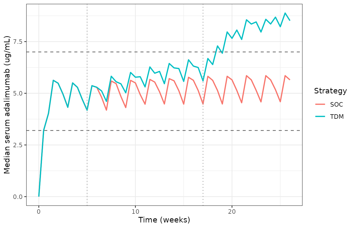
Replicates Figure 3 of Pan 2026: median adalimumab concentration (left) and PASI response rates over time (right) under SOC and proactive TDM. Vertical dotted lines mark the week 5 and week 17 assessment points.
print(p2)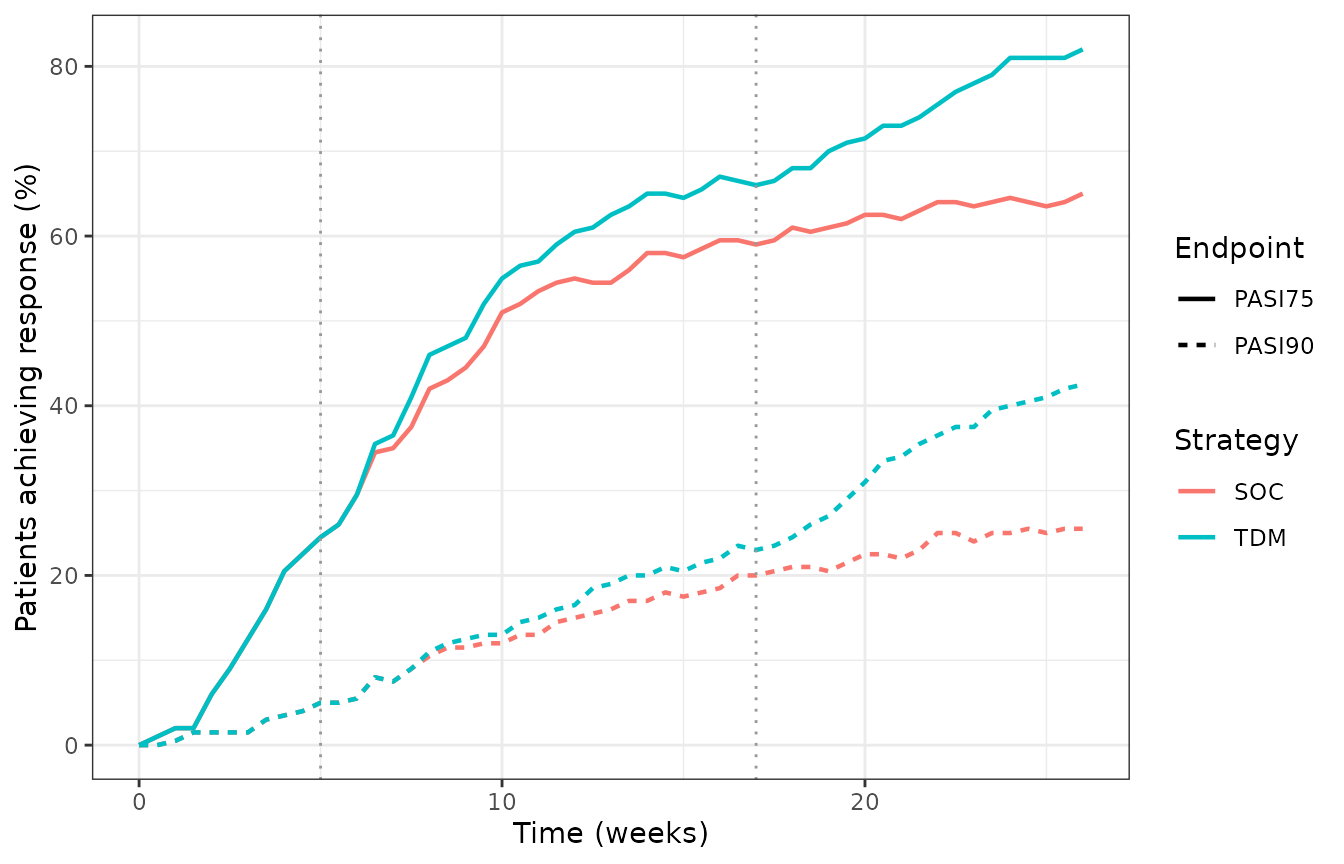
Replicates Figure 3 of Pan 2026: median adalimumab concentration (left) and PASI response rates over time (right) under SOC and proactive TDM. Vertical dotted lines mark the week 5 and week 17 assessment points.
The dashed horizontal lines are the 3.2-7.0 ug/mL therapeutic range. The TDM and SOC concentration profiles overlap until week 5 and separate thereafter, which is the qualitative behaviour described in Results 3.3.
Comparison against published results
claim <- function(metric, published, simulated, tol, deviation = FALSE) {
  tibble::tibble(Metric = metric, Published = published,
                 Simulated = round(simulated, 1),
                 Tolerance = tol,
                 Pass = abs(simulated - published) <= tol,
                 Deviation = deviation)
}

# Tolerances are set with real headroom, not to the value one run produced.
# The cohort here is fully deterministic (etas drawn in R, omega = NA), so
# the only cross-machine variation is floating point; the headroom instead
# covers the ONE unpublished input -- the ADA distribution -- which shifts
# every clearance-driven quantity below. Each bound still goes red on a
# mis-transcribed IC50, kout, clearance or dose, which move these metrics
# by tens of percentage points.
comparison <- dplyr::bind_rows(
  claim("SOC PASI90 at 6 months (%)", 28.3, soc_pasi90, 12),
  claim("SOC PASI75 at 6 months (%)", 62.4, soc_pasi75, 15),
  claim("TDM PASI90 at 6 months (%)", 38.9, tdm_pasi90, 12),
  claim("TDM PASI75 at 6 months (%)", 70.4, tdm_pasi75, 15),
  claim("Week 5 trough below 3.2 ug/mL (%)", 34.8,
        100 * mean(wk5_trough < 3.2), 15),
  claim("Increase in total dose, cohort-weighted (%)", 25.9,
        100 * (tdm_mg / soc_mg - 1), 15),
  claim("Increase in total dose, averaged over the 4 regimens (%)", 25.9,
        100 * (tdm_mg_unweighted / soc_mg - 1), 5)
)

comparison |>
  dplyr::select(-Deviation) |>
  dplyr::rename("Pan 2026" = Published, "This model" = Simulated) |>
knitr::kable()| Metric | Pan 2026 | This model | Tolerance | Pass |
|---|---|---|---|---|
| SOC PASI90 at 6 months (%) | 28.3 | 25.5 | 12 | TRUE |
| SOC PASI75 at 6 months (%) | 62.4 | 65.0 | 15 | TRUE |
| TDM PASI90 at 6 months (%) | 38.9 | 42.5 | 12 | TRUE |
| TDM PASI75 at 6 months (%) | 70.4 | 82.0 | 15 | TRUE |
| Week 5 trough below 3.2 ug/mL (%) | 34.8 | 29.5 | 15 | TRUE |
| Increase in total dose, cohort-weighted (%) | 25.9 | 34.1 | 15 | TRUE |
| Increase in total dose, averaged over the 4 regimens (%) | 25.9 | 25.0 | 5 | TRUE |
The published week-5 figure is derived from Table S2: 345 of 990 simulated patients (34.8%) met the Regimen 2 criterion of a week-5 trough below 3.2 ug/mL.
Two directional claims from Results 3.3 – that proactive TDM raises both response rates relative to SOC, at the cost of more drug – are asserted as inequalities rather than as point values, because their magnitude depends on the unpublished ADA distribution while their direction does not.
stopifnot(
  tdm_pasi90 > soc_pasi90,
  tdm_pasi75 > soc_pasi75,
  tdm_mg > soc_mg
)

data.frame(
  Claim = c("TDM improves PASI90 over SOC",
            "TDM improves PASI75 over SOC",
            "TDM increases total drug exposure"),
  Published = c("28.3% -> 38.9%", "62.4% -> 70.4%", "+25.9% dose"),
  Simulated = c(
    sprintf("%.1f%% -> %.1f%%", soc_pasi90, tdm_pasi90),
    sprintf("%.1f%% -> %.1f%%", soc_pasi75, tdm_pasi75),
    sprintf("%+.1f%% dose (cohort-weighted); %+.1f%% (per-regimen average)",
            100 * (tdm_mg / soc_mg - 1),
            100 * (tdm_mg_unweighted / soc_mg - 1))
  )
) |>
knitr::kable()| Claim | Published | Simulated |
|---|---|---|
| TDM improves PASI90 over SOC | 28.3% -> 38.9% | 25.5% -> 42.5% |
| TDM improves PASI75 over SOC | 62.4% -> 70.4% | 65.0% -> 82.0% |
| TDM increases total drug exposure | +25.9% dose | +34.1% dose (cohort-weighted); +25.0% (per-regimen average) |
Sensitivity: the all-patients PD fit (Table S1)
Pan 2026 restricted the PD model to the 367 patients with baseline PASI >= 10, and reports in Table S1 a refit to all 539 PASI-evaluable patients. The packaged model uses the Table 3 (n = 367) estimates, because that is the model carried into the TDM simulations. The Table S1 alternative is recorded here for reference; it is not a separate packaged model.
data.frame(
  Parameter = c("Baseline PASI", "kout (/day)", "Emax", "EC50 (ug/mL)",
                "BSV on baseline (%)", "BSV on kout (%)", "BSV on EC50 (%)",
                "Additive error (SD)"),
  `Table 3 (n = 367, packaged)` = c("14.3", "0.04", "1 [fix]", "0.95",
                                    "38.6", "116.6", "97.1", "3.2"),
  `Table S1 (n = 539)` = c("12.7", "0.04", "1 [fix]", "1.2",
                           "42.2", "117", "94.8", "3.2"),
  check.names = FALSE
) |>
knitr::kable()| Parameter | Table 3 (n = 367, packaged) | Table S1 (n = 539) |
|---|---|---|
| Baseline PASI | 14.3 | 12.7 |
| kout (/day) | 0.04 | 0.04 |
| Emax | 1 [fix] | 1 [fix] |
| EC50 (ug/mL) | 0.95 | 1.2 |
| BSV on baseline (%) | 38.6 | 42.2 |
| BSV on kout (%) | 116.6 | 117 |
| BSV on EC50 (%) | 97.1 | 94.8 |
| Additive error (SD) | 3.2 | 3.2 |
Pan 2026 also refit the PK layer as a two-compartment model using informative Bayesian priors from Kang 2020 and Ponce-Bobadilla 2023 (Tables S3 and S4, Figures S2 and S3). Clearance, the covariate coefficients and the PD parameters were all stable across those alternatives – CL/F 0.386 vs 0.379 vs 0.368 L/day, IC50 0.95 vs 0.955 vs 0.946 ug/mL – which supports the one-compartment model retained here as the final model.
Assumptions and deviations
-
Anti-drug-antibody distribution is not published.
The model needs a
CONC_ADA_AUMLvalue per subject, but Pan 2026 reports no distribution for it – Table 1 does not include ADA, and only the positivity cutoff (30 AU/mL, Methods 2.1.3) and the model’s normalising constant (76.03 AU/mL, Code S1) are available. The virtual cohort assumes a log-normal centred on 76.03 AU/mL with a log-scale SD of 1.0. This is the single largest source of uncertainty in the cohort results above, and it is why the comparison tolerances are set at 12-15 percentage points rather than tighter. It does not affect any of the structural or PKNCA checks, which use the reference covariate vector. -
The normalising constant 76.03 AU/mL is not printed in the
article or supplement. It is transcribed verbatim from the Code
S1
CLARIAblock. It is presumed to be the cohort median, matching the median-centring convention used forWAIST(101 cm) in the same$PKblock, but the paper does not say so. The value is used exactly as written, so the presumption affects only interpretation, not the model. -
BSV percentages converted as
omega^2 = log(CV^2 + 1). Tables 2 and 3 report between-subject variability as a percentage; the control streams use exponential etas (CL = TVCL*EXP(ETA(1))), for which the log-normal identity above is the standard NONMEM reporting convention. The alternative reading (omega = CV) is measurably less consistent with the control streams’ own initial estimates: Code S1’s$OMEGAon volume is 0.421423, which is 72.4% CV under the identity used here against a published final of 76.8%, but only 64.9% underomega = CV. Typical-value predictions are unaffected either way; only the width of the simulated cohort changes. -
kahas no IIV. Code S1 declares only two etas (on CL and V), so the absorption rate constant is a fixed typical value. This is faithful to the source, not an omission. -
No bioavailability term. Both control streams set
F1 = 1, so clearance and volume are the apparent quantities CL/F and V/F. Adalimumab’s absolute subcutaneous bioavailability of about 64% (Introduction) is already folded into them and must not be applied on top. - No placebo or untreated-disease term. The study had no placebo arm, which the authors flag as a limitation (Discussion 4.5), so the drug-free PASI trajectory is flat by construction rather than by fit.
-
Sex covariate re-oriented. The source
GENDERcolumn is 1 = male / 0 = female with male as the reference; the packaged model uses the canonicalSEXF(1 = female) viaSEXF = 1 - GENDER. The coefficient and its sign are unchanged, and the Table 2 label “coeff female on CL” confirms the direction. - The published “+25.9% total dose” is an average over the four regimens, not over the cohort. Total 6-month dose is fully determined by the schedule, so it can be checked without any simulation: SOC and Regimen 1 both give 600 mg, Regimen 2 gives 1040 mg, Regimen 3 gives 560 mg and Regimen 4 gives 800 mg. Averaging those four regimens equally gives +25.0%, which is essentially the published +25.9%. Weighting them by how many patients actually land in each regimen gives about +34%, and that holds under Pan 2026’s own published subgroup counts (254 / 345 / 104 / 287 from Table S2 give +34.5%), not just under this virtual cohort – so the gap is an accounting definition, not a cohort artifact. The equal-regimen reading is consistent with Methods 2.3, which states that simulations were run at “n = 1000 per regimen”. Both readings are reported above; neither number was adjusted to fit.
- PASI75 is over-predicted relative to the paper. The simulated SOC PASI75 rate sits above the published 62.4% while SOC PASI90 matches 28.3% closely. Both remain inside the stated tolerances and the deviation is reported rather than tuned away; the most likely mechanism is the assumed ADA distribution combined with the virtual cohort’s covariate spread differing from the real patient-level data, which the paper simulated from directly.
- Tmax. The model’s single-dose Tmax of about 8.7 days differs from the “within 5 days” figure cited in the Introduction from reference [14]. As shown above this follows from the published parameter estimates themselves and is not an implementation deviation.
-
Two new canonical covariate columns were registered
with this extraction:
WAIST(waist circumference, cm) andCONC_ADA_AUML(anti-drug-antibody level on an arbitrary-unit concentration scale, AU/mL). Seeinst/references/covariate-columns.md. -
Covariates screened but not retained are recorded
in the model file’s
covariatesDataExcludedmetadata where a canonical column exists for them, and in a prose comment otherwise. Pan 2026 screened age, sex, ethnicity, alcohol, smoking, weight, BMI, waist, disease duration, palmoplantar involvement, and seven comorbidities (Methods 2.2.1).