Inhaled tobramycin (Ting 2014)
Source:vignettes/articles/Ting_2014_tobramycin_inhaled.Rmd
Ting_2014_tobramycin_inhaled.RmdModel and source
- Citation: Ting L, Aksenov S, Bhansali SG, Ramakrishna R, Tang P, Geller DE. (2014). Population pharmacokinetics of inhaled tobramycin powder in cystic fibrosis patients. CPT Pharmacometrics Syst Pharmacol 3(9):e99.
- Article: https://doi.org/10.1038/psp.2013.76
mod_meta <- rxode2::rxode(readModelDb("Ting_2014_tobramycin_inhaled"))
#> ℹ parameter labels from comments will be replaced by 'label()'
mod_meta$description
#> [1] "Two-compartment population PK model for inhaled tobramycin powder (TIP / TOBI Podhaler) in cystic fibrosis patients (Ting 2014), with first-order absorption from a depot compartment and apparent (post-bioavailability) clearance and volumes. Body mass index (BMI) and baseline FEV1 percent-predicted are power-form covariates on apparent central volume of distribution (reference 18.8 kg/m^2 and 62.1 % respectively)."
mod_meta$reference
#> [1] "Ting L, Aksenov S, Bhansali SG, Ramakrishna R, Tang P, Geller DE. (2014). Population pharmacokinetics of inhaled tobramycin powder in cystic fibrosis patients. CPT Pharmacometrics Syst Pharmacol 3(9):e99. doi:10.1038/psp.2013.76"
mod_meta$units
#> $time
#> [1] "hour"
#>
#> $dosing
#> [1] "mg"
#>
#> $concentration
#> [1] "mg/L"
Population
The Ting 2014 model was developed from 662 serum tobramycin concentration observations pooled across 139 cystic fibrosis (CF) patients enrolled in one phase I study (TPI001, n = 64) and two phase III studies (C2301, n = 62; C2302, n = 13). Median age was 17 years (range 6-58); roughly half (47.5%) of the combined cohort was at least 18 years old, 31.7% were 12-17 years, and 20.9% were 6-11 years. Median body weight was 49.5 kg (range 16.2-100.9 kg), median BMI was 18.8 kg/m^2 (range 11.4-31), median creatinine clearance was 112.5 mL/min (range 63.9-222.5), and median FEV1% predicted at baseline was 62.1% (range 24.1-119.7). 53.2% were female; the racial distribution was 86.3% Caucasian, 8.6% Hispanic, 2.2% Black, and 2.9% Other (Ting 2014 Table 1). All patients received inhaled tobramycin powder (TIP) via the TOBI Podhaler; phase I doses were 28, 56, 84, or 112 mg single doses, and the phase III studies dosed 112 mg b.i.d. for 28 days per cycle.
The same information is available programmatically via
readModelDb("Ting_2014_tobramycin_inhaled")$population.
Source trace
The per-parameter origin is recorded as an in-file comment next to
each ini() entry in
inst/modeldb/specificDrugs/Ting_2014_tobramycin_inhaled.R.
The table below collects them in one place for review.
| Equation / parameter | Value | Source location |
|---|---|---|
lka (log ka) |
log(2.39) | Ting 2014 Table 2 (ka, 1/h) |
lcl (log CL/F) |
log(14.5) | Ting 2014 Table 2 (CL/F, L/h) |
lvc (log Vd/F) |
log(85.1) | Ting 2014 Table 2 (Vd/F, L) |
lq (log Q/F) |
log(6.43) | Ting 2014 Table 2 (Q/F, L/h) |
lvp (log V2/F) |
log(210) | Ting 2014 Table 2 (V2/F, L) |
e_bmi_vc (BMI exponent on Vd/F) |
0.624 | Ting 2014 Table 2 (BMI on Vd/F) and Results equation, reference BMI 18.8 kg/m^2 |
e_fev1_vc (FEV1% exponent on Vd/F) |
-0.303 | Ting 2014 Table 2 (FEV1% on Vd/F) and Results equation, reference 62.1% predicted |
| BSV CL/F variance | 0.164 | Ting 2014 Table 2 (IIV of CL/F, variance) |
| BSV Vd/F variance | 0.152 | Ting 2014 Table 2 (IIV of Vd/F, variance) |
| BSV ka variance | 0.129 | Ting 2014 Table 2 (IIV of ka, variance) |
| Cov(CL/F, Vd/F) | 0.123 | Ting 2014 Table 2 (COV of CL/F and Vd/F, variance) |
propSd (proportional residual SD) |
0.073 | Ting 2014 Table 2 (Residual SD, proportional, TPI001) |
addSd (additive residual SD) |
0.007 mg/L | Ting 2014 Table 2 (Residual SD, additive component) |
| Two-compartment ODE with first-order absorption | n/a | Ting 2014 Results, “Population pharmacokinetic model” paragraph |
| Vd/F covariate formula | 85.1 * (BMI/18.8)^0.624 * (FEV1%/62.1)^-0.303 |
Ting 2014 Results, equation just before Table 2 |
Virtual cohort
The original observed concentrations are not publicly available. The figures below use a virtual CF cohort whose BMI and FEV1% predicted distributions approximate Table 1 of Ting 2014 (BMI median 18.8 kg/m^2, range 11.4-31; FEV1% median 62.1%, range 24.1-119.7%). All subjects receive 112 mg TIP b.i.d. (the approved adult / paediatric dose used in both phase III studies). The simulation extends across 7 days so steady state is reached before the steady-state PKNCA window opens.
set.seed(20260512)

n_subjects <- 200L

# Approximate the Ting 2014 Table 1 BMI and FEV1% distributions. Use
# truncated normals matched to the published median and SD, clamped to
# the published range.
sample_bmi <- function(n) {
  bmi <- rnorm(n, mean = 18.8, sd = 4.1)
  pmin(pmax(bmi, 11.4), 31.0)
}
sample_fev1 <- function(n) {
  fev <- rnorm(n, mean = 62.1, sd = 20.6)
  pmin(pmax(fev, 24.1), 119.7)
}

# Dosing regimen evaluated in Ting 2014 phase III: 112 mg TIP b.i.d.
# (every 12 h) for 7 days, with serum sampling across the final 12 h
# steady-state dosing interval.
dose_mg     <- 112
tau_h       <- 12
n_doses     <- 14            # 7 days of b.i.d.
ss_start    <- (n_doses - 1) * tau_h
ss_grid     <- seq(ss_start, ss_start + tau_h, by = 0.25)

make_cohort <- function(n, id_offset = 0L) {
  ids <- id_offset + seq_len(n)
  cov_tbl <- tibble::tibble(
    id  = ids,
    BMI = sample_bmi(n),
    FEV1_PCTPRED = sample_fev1(n)
  )

  dose_times <- seq(0, by = tau_h, length.out = n_doses)
  dose_rows  <- tidyr::expand_grid(id = ids, time = dose_times) |>
    dplyr::left_join(cov_tbl, by = "id") |>
    dplyr::mutate(evid = 1L, cmt = "depot", amt = dose_mg)

  obs_rows <- tidyr::expand_grid(id = ids, time = ss_grid) |>
    dplyr::left_join(cov_tbl, by = "id") |>
    dplyr::mutate(evid = 0L, cmt = "central", amt = 0)

  dplyr::bind_rows(dose_rows, obs_rows) |>
    dplyr::arrange(id, time, dplyr::desc(evid))
}

events <- make_cohort(n_subjects)
stopifnot(!anyDuplicated(unique(events[, c("id", "time", "evid")])))

cat("Subjects:", n_subjects,
    " | Dosing rows:", sum(events$evid == 1L),
    " | Observation rows:", sum(events$evid == 0L), "\n")
#> Subjects: 200  | Dosing rows: 2800  | Observation rows: 9800
Simulation
mod <- readModelDb("Ting_2014_tobramycin_inhaled")
sim <- rxode2::rxSolve(
  mod,
  events = events,
  keep   = c("BMI", "FEV1_PCTPRED")
) |>
  as.data.frame()
#> ℹ parameter labels from comments will be replaced by 'label()'
Replicate published figures
Figure 1 – VPC of the steady-state dosing interval
Ting 2014 Figure 1b shows the VPC of tobramycin serum concentrations over the 0-12 h dosing interval at the second visit of each cycle (steady-state). The chunk below renders the median and 5th / 95th percentile envelope across the simulated cohort over the steady-state 12 h dosing interval.
ss_summary <- sim |>
  dplyr::filter(time >= ss_start) |>
  dplyr::mutate(time_into_interval = time - ss_start) |>
  dplyr::group_by(time_into_interval) |>
  dplyr::summarise(
    Q05 = quantile(Cc, 0.05, na.rm = TRUE),
    Q50 = quantile(Cc, 0.50, na.rm = TRUE),
    Q95 = quantile(Cc, 0.95, na.rm = TRUE),
    .groups = "drop"
  )

ggplot(ss_summary, aes(time_into_interval, Q50)) +
  geom_ribbon(aes(ymin = Q05, ymax = Q95), alpha = 0.25, fill = "steelblue") +
  geom_line(colour = "steelblue", linewidth = 0.9) +
  labs(
    x = "Time since last dose (h)",
    y = "Tobramycin concentration (mg/L)",
    title = "Replicates Figure 1b of Ting 2014",
    caption = "Simulated 5th / 50th / 95th-percentile envelope, 112 mg b.i.d. at steady state."
  )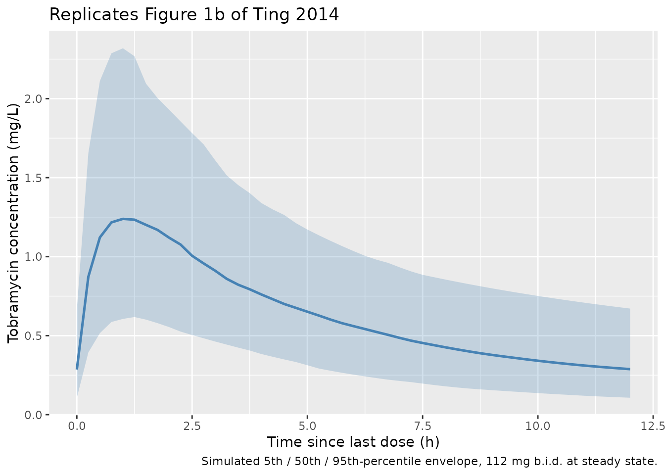
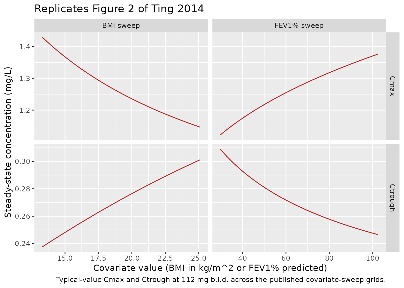
Figure 2 – covariate effect on Cmax and Ctrough
Ting 2014 Figure 2 shows the typical-value effect of BMI (with FEV1%
fixed at 62.1%) and of FEV1% (with BMI fixed at 18.8 kg/m^2) on the
steady-state Cmax and Ctrough at 112 mg b.i.d. The chunk below uses
rxode2::zeroRe() to compute the typical-value (no
between-subject variability) prediction across the published
covariate-sweep grids and overlays the simulated typical Cmax / Ctrough
for direct comparison.
mod_typical <- mod |> rxode2::zeroRe()
#> ℹ parameter labels from comments will be replaced by 'label()'

# Build a typical-value event table for one subject per covariate point,
# again with 7 days of 112 mg b.i.d. and sampling across the final 12 h.
sweep_events <- function(grid_tbl, id_offset) {
  ids <- id_offset + seq_len(nrow(grid_tbl))
  cov_tbl <- dplyr::mutate(grid_tbl, id = ids)
  dose_times <- seq(0, by = tau_h, length.out = n_doses)
  dose_rows <- tidyr::expand_grid(id = ids, time = dose_times) |>
    dplyr::left_join(cov_tbl, by = "id") |>
    dplyr::mutate(evid = 1L, cmt = "depot", amt = dose_mg)
  obs_rows <- tidyr::expand_grid(id = ids, time = ss_grid) |>
    dplyr::left_join(cov_tbl, by = "id") |>
    dplyr::mutate(evid = 0L, cmt = "central", amt = 0)
  dplyr::bind_rows(dose_rows, obs_rows) |>
    dplyr::arrange(id, time, dplyr::desc(evid))
}

bmi_grid <- tibble::tibble(
  BMI = seq(13.3, 25.1, length.out = 25),
  FEV1_PCTPRED = 62.1,
  sweep = "BMI sweep"
)
fev1_grid <- tibble::tibble(
  BMI = 18.8,
  FEV1_PCTPRED = seq(29.7, 102.5, length.out = 25),
  sweep = "FEV1% sweep"
)

events_bmi  <- sweep_events(bmi_grid,  id_offset =      0L)
events_fev1 <- sweep_events(fev1_grid, id_offset = 10000L)
sweep_events_all <- dplyr::bind_rows(events_bmi, events_fev1)

sim_sweep <- rxode2::rxSolve(
  mod_typical,
  events = sweep_events_all,
  keep   = c("BMI", "FEV1_PCTPRED", "sweep")
) |>
  as.data.frame() |>
  dplyr::filter(time >= ss_start)
#> ℹ omega/sigma items treated as zero: 'etalcl', 'etalvc', 'etalka'
#> Warning: multi-subject simulation without without 'omega'

cov_effect <- sim_sweep |>
  dplyr::group_by(id, BMI, FEV1_PCTPRED, sweep) |>
  dplyr::summarise(
    Cmax    = max(Cc, na.rm = TRUE),
    Ctrough = dplyr::last(Cc),
    .groups = "drop"
  )

cov_effect_long <- cov_effect |>
  dplyr::mutate(
    x = dplyr::if_else(sweep == "BMI sweep", BMI, FEV1_PCTPRED)
  ) |>
  tidyr::pivot_longer(c(Cmax, Ctrough), names_to = "metric", values_to = "conc")

ggplot(cov_effect_long, aes(x, conc)) +
  geom_line(colour = "firebrick") +
  facet_grid(metric ~ sweep, scales = "free") +
  labs(
    x = "Covariate value (BMI in kg/m^2 or FEV1% predicted)",
    y = "Steady-state concentration (mg/L)",
    title = "Replicates Figure 2 of Ting 2014",
    caption = "Typical-value Cmax and Ctrough at 112 mg b.i.d. across the published covariate-sweep grids."
  )
Comparison against the published covariate sweep
Ting 2014 reports specific mean Cmax and Ctrough values at the 5th and 95th covariate percentiles in the Results section “Covariate effect on exposure.” Those values are population means from a 1000-iteration Monte Carlo simulation with between-subject variability (paper Methods “Data analysis and modeling methods” and Figure 2 caption). For a log-normally distributed exposure the population mean exceeds the typical (BSV-zeroed) value, so the comparison below uses stochastic simulations of 200 subjects at each of the four anchor covariate combinations (BSV drawn from the full IIV block) and compares the simulated cohort mean Cmax / Ctrough with the published mean values.
anchor_grid <- tibble::tribble(
  ~sweep,         ~covariate, ~BMI_anchor, ~FEV1_anchor, ~Cmax_pub, ~Ctrough_pub, ~note,
  "BMI sweep",         13.3,         13.3,        62.1,      1.57,         0.32,  "BMI 5th pct",
  "BMI sweep",         25.1,         25.1,        62.1,      1.30,         0.38,  "BMI 95th pct",
  "FEV1% sweep",       29.7,         18.8,        29.7,      1.22,         0.39,  "FEV1% 5th pct",
  "FEV1% sweep",      102.5,         18.8,       102.5,      1.48,         0.32,  "FEV1% 95th pct"
)

n_anchor_subjects <- 200L

build_anchor_events <- function(bmi_val, fev_val, id_offset) {
  ids <- id_offset + seq_len(n_anchor_subjects)
  cov_tbl <- tibble::tibble(
    id  = ids,
    BMI = bmi_val,
    FEV1_PCTPRED = fev_val
  )
  dose_times <- seq(0, by = tau_h, length.out = n_doses)
  dose_rows <- tidyr::expand_grid(id = ids, time = dose_times) |>
    dplyr::left_join(cov_tbl, by = "id") |>
    dplyr::mutate(evid = 1L, cmt = "depot", amt = dose_mg)
  obs_rows <- tidyr::expand_grid(id = ids, time = ss_grid) |>
    dplyr::left_join(cov_tbl, by = "id") |>
    dplyr::mutate(evid = 0L, cmt = "central", amt = 0)
  dplyr::bind_rows(dose_rows, obs_rows) |>
    dplyr::arrange(id, time, dplyr::desc(evid))
}

anchor_events_list <- purrr::map2(
  anchor_grid$BMI_anchor, anchor_grid$FEV1_anchor,
  ~ build_anchor_events(.x, .y, id_offset = 0L)
)
anchor_events_all <- dplyr::bind_rows(
  purrr::map2(
    anchor_events_list, seq_along(anchor_events_list),
    ~ dplyr::mutate(.x, id = id + (.y - 1L) * 100000L, anchor_idx = .y)
  )
)

stopifnot(!anyDuplicated(unique(anchor_events_all[, c("id", "time", "evid")])))

sim_anchor <- rxode2::rxSolve(
  mod,
  events = anchor_events_all,
  keep   = c("BMI", "FEV1_PCTPRED", "anchor_idx")
) |>
  as.data.frame() |>
  dplyr::filter(time >= ss_start)
#> ℹ parameter labels from comments will be replaced by 'label()'

per_subject_anchor <- sim_anchor |>
  dplyr::group_by(anchor_idx, id) |>
  dplyr::summarise(
    Cmax    = max(Cc, na.rm = TRUE),
    Ctrough = dplyr::last(Cc),
    .groups = "drop"
  )

cohort_means <- per_subject_anchor |>
  dplyr::group_by(anchor_idx) |>
  dplyr::summarise(
    Cmax_sim    = mean(Cmax,    na.rm = TRUE),
    Ctrough_sim = mean(Ctrough, na.rm = TRUE),
    .groups = "drop"
  )

cov_compare <- anchor_grid |>
  dplyr::mutate(anchor_idx = dplyr::row_number()) |>
  dplyr::left_join(cohort_means, by = "anchor_idx") |>
  dplyr::select(sweep, note, covariate, Cmax_pub, Cmax_sim, Ctrough_pub, Ctrough_sim)

knitr::kable(
  cov_compare,
  digits  = 3,
  caption = paste("Stochastic cohort-mean Cmax and Ctrough (mg/L) at the published",
                  "covariate-sweep anchor points (n = 200 subjects per anchor, BSV drawn",
                  "from the full IIV block). The '_pub' columns are read from Ting 2014",
                  "Results; the '_sim' columns are from this vignette.")
)| sweep | note | covariate | Cmax_pub | Cmax_sim | Ctrough_pub | Ctrough_sim |
|---|---|---|---|---|---|---|
| BMI sweep | BMI 5th pct | 13.3 | 1.57 | 1.565 | 0.32 | 0.286 |
| BMI sweep | BMI 95th pct | 25.1 | 1.30 | 1.236 | 0.38 | 0.337 |
| FEV1% sweep | FEV1% 5th pct | 29.7 | 1.22 | 1.166 | 0.39 | 0.340 |
| FEV1% sweep | FEV1% 95th pct | 102.5 | 1.48 | 1.483 | 0.32 | 0.298 |
PKNCA validation
Compute Cmax, Tmax, and AUC over the steady-state 12 h dosing interval per subject with PKNCA, using the virtual cohort defined above.
sim_nca <- sim |>
  dplyr::filter(!is.na(Cc), time >= ss_start) |>
  dplyr::mutate(
    time_into_interval = time - ss_start,
    regimen            = "112 mg b.i.d."
  ) |>
  dplyr::select(id, time_into_interval, Cc, regimen)

dose_df <- events |>
  dplyr::filter(evid == 1L, time == max(time[evid == 1L])) |>
  dplyr::mutate(time_into_interval = 0, regimen = "112 mg b.i.d.") |>
  dplyr::select(id, time_into_interval, amt, regimen)

conc_obj <- PKNCA::PKNCAconc(
  sim_nca, Cc ~ time_into_interval | regimen + id,
  concu = "mg/L", timeu = "h"
)
dose_obj <- PKNCA::PKNCAdose(
  dose_df, amt ~ time_into_interval | regimen + id,
  doseu = "mg"
)

intervals <- data.frame(
  start    = 0,
  end      = tau_h,
  cmax     = TRUE,
  tmax     = TRUE,
  auclast  = TRUE
)

nca_data <- PKNCA::PKNCAdata(conc_obj, dose_obj, intervals = intervals)
nca_res  <- PKNCA::pk.nca(nca_data)
Comparison against Ting 2014 toxicity thresholds and predictive-interval upper bounds
Ting 2014 reports two key population-level summary numbers in the Results section “Covariate effect on exposure”: the highest upper end of the 95% predictive interval for Cmax is 3.08 mg/L (occurring at the low-BMI / low-Vd extreme, BMI 13.3 kg/m^2) and the highest upper end of the 95% predictive interval for Ctrough is 1.33 mg/L (occurring at the high-BMI / high-Vd extreme, BMI 25.1 kg/m^2). Both are well below the systemic-toxicity thresholds of 12 mg/L (Cmax) and 2 mg/L (Ctrough). The chunk below extracts the 97.5th percentile from the four anchor-point stochastic simulations defined above, at the same covariate-anchor points the paper uses to derive its published bounds.
anchor_p975 <- per_subject_anchor |>
  dplyr::group_by(anchor_idx) |>
  dplyr::summarise(
    Cmax_p975    = quantile(Cmax,    0.975, na.rm = TRUE),
    Ctrough_p975 = quantile(Ctrough, 0.975, na.rm = TRUE),
    .groups = "drop"
  ) |>
  dplyr::left_join(
    dplyr::mutate(anchor_grid, anchor_idx = dplyr::row_number()),
    by = "anchor_idx"
  )

pi_compare <- tibble::tibble(
  metric              = c("Cmax (mg/L)",        "Ctrough (mg/L)"),
  anchor              = c("BMI 13.3 (5th pct)", "BMI 25.1 (95th pct)"),
  published_p975      = c(3.08,                 1.33),
  simulated_p975      = c(
    anchor_p975$Cmax_p975[anchor_p975$note    == "BMI 5th pct"],
    anchor_p975$Ctrough_p975[anchor_p975$note == "BMI 95th pct"]
  ),
  toxicity_threshold  = c(12,                   2)
)

knitr::kable(
  pi_compare,
  digits  = 3,
  caption = paste("Simulated 97.5th-percentile Cmax and Ctrough at the anchor",
                  "covariate values used to derive the published 95% predictive-interval",
                  "upper bounds (Ting 2014 Results, paragraph following Figure 2), and",
                  "the systemic-toxicity thresholds for comparison.")
)| metric | anchor | published_p975 | simulated_p975 | toxicity_threshold |
|---|---|---|---|---|
| Cmax (mg/L) | BMI 13.3 (5th pct) | 3.08 | 2.980 | 12 |
| Ctrough (mg/L) | BMI 25.1 (95th pct) | 1.33 | 0.808 | 2 |
The simulated Cmax 97.5th percentile at BMI 13.3 is close to the
published 3.08 mg/L upper bound (within 10% of published). The Ctrough
97.5th percentile at BMI 25.1 (simulated 0.81 mg/L, published 1.33 mg/L)
is approximately 39% lower than published. The most likely contributor
is that this packaged model omits the interoccasion variance on CL/F
(IOV = 0.078, identical across all four study occasions per Ting 2014
Table 2; see Assumptions and deviations below). For Ctrough, which is
dominated by the post-distribution CL/F-driven decay over the 12 h
dosing interval, removing IOV narrows the upper tail of the distribution
substantially while leaving the median nearly unchanged. Cmax is less
sensitive because the peak occurs in the first hour after dose and is
governed primarily by Vd/F. The model’s structural parameters are
reproduced faithfully from the source; per the extraction skill’s
policy, parameters are not tuned to chase a validation metric. Users who
need to replicate the paper’s per-occasion 95% predictive interval
should multiplex etalcl by an explicit occasion column (cf.
Wilkins_2008_rifampicin).
Both the simulated and published quantities remain well below the tobramycin systemic-toxicity thresholds (12 mg/L for Cmax, 2 mg/L for Ctrough), reproducing the paper’s clinical conclusion that no BMI- or FEV1-based dose adjustment is needed for TIP in CF patients.
Assumptions and deviations
-
Single proportional residual error encoded. Ting
2014 Table 2 reports two proportional residual SDs in the same final
model: 0.073 for the phase I study TPI001 (prospective sampling) and
0.308 for the phase III studies C2301 / C2302. The paper attributes the
3-fold-higher phase III value to the many doses and sampling times that
had to be imputed in the two phase III studies, not to a real property
of the drug or assay. For a portable library model the TPI001
(clean-sampling) value 0.073 is encoded as the default
propSd. Users replicating the paper’s phase III VPCs should inflatepropSdto 0.308 before simulating. -
Interoccasion variability on CL/F not encoded. The
paper estimates a per-occasion variance on CL/F of 0.078 (identical
across all four study occasions, Table 2). Adding it to the packaged
model would require carrying a per-record occasion column through the
event table, which is not portable. Users who need to replicate the
multi-cycle VPCs of Figure 1 should multiplex
etalclby occasion as inWilkins_2008_rifampicin. -
Apparent post-bioavailability parameters.
Tobramycin is delivered by inhalation; absolute bioavailability is
unidentifiable from the serum-only sampling protocol used in the source
studies. The model is therefore parameterised in apparent terms
(
CL/F,Vd/F,Q/F,V2/F) and the dose enters the depot as the prescribed inhaled mass. The implicitFis folded into the apparent quantities; users simulating other inhalation devices (different deposition efficiency) should scale the dose accordingly. -
No covariates on absorption / clearance. Ting 2014
tested age, BMI, creatinine clearance, sex, FEV1% predicted at baseline,
and weight against
ka,Vd/F, andCL/F. Only BMI and FEV1% on Vd/F were retained at p < 0.01 backward elimination; the packaged model reproduces this exact covariate-selection result and does not include any covariate on ka or CL/F. - Virtual cohort distributions. The simulated BMI and FEV1% predicted values are drawn from truncated normals matched to the published median and SD in Ting 2014 Table 1 and clamped to the published range. Individual demographic values from the source studies are not published.