Voriconazole (Muto 2015)
Source:vignettes/articles/Muto_2015_voriconazole.Rmd
Muto_2015_voriconazole.RmdModel and source
- Citation: Muto C, Shoji S, Tomono Y, Liu P. Population pharmacokinetic analysis of voriconazole from a pharmacokinetic study with immunocompromised Japanese pediatric subjects. Antimicrob Agents Chemother. 2015;59(6):3216-3223. doi:10.1128/AAC.04993-14
- Description: Two-compartment population pharmacokinetic model with first-order absorption (lag time, oral bioavailability) and parallel linear plus time-dependent Michaelis-Menten elimination for voriconazole in 21 immunocompromised Japanese pediatric subjects (Muto 2015). Vmax declines with time after the first dose toward Vmax * (1 - Vmax_inh) with half-time T50; the maximum inhibition fraction Vmax_inh is fixed to 1 (full inhibition) for CYP2C19 heterozygous-extensive-metabolizer or poor-metabolizer subjects and modeled on the logit scale otherwise. Allometric scaling on all clearances (exponent 0.75) and all volumes (exponent 1) to a 70 kg reference; oral bioavailability F1 is modeled on the logit scale with a Manly-transformed log-normal random effect.
- Article: Antimicrob Agents Chemother. 2015;59(6):3216-3223
Population
Muto 2015 fitted a population PK model to 276 voriconazole plasma concentrations collected from 21 immunocompromised Japanese pediatric subjects (9 male, 12 female; age 3-14 years, median 10; body weight 11.5-55.2 kg, median 31.5) enrolled at six centres in Japan (Table 2). The CYP2C19 genotype distribution was 9 extensive metabolizers (EM, 43%), 10 heterozygous extensive metabolizers (HEM, 48%), and 2 poor metabolizers (PM, 9.5%). All subjects received the intravenous (i.v.) regimen on days 1-7; 18 of 21 continued on to the oral regimen on days 8-14. Three age / weight strata received different doses (Table 1):
- Children 2 to <12 yr and adolescents 12 to <15 yr with body weight <50 kg (“Peds + Adol 1”): 9 mg/kg i.v. q12h loading on day 1, 8 mg/kg i.v. q12h maintenance on days 2-7, 9 mg/kg p.o. q12h (capped at 350 mg per dose) on days 8-14.
- Adolescents 12 to <15 yr with body weight >=50 kg (“Adol 2”): 6 mg/kg i.v. q12h loading on day 1, 4 mg/kg i.v. q12h maintenance on days 2-7, 200 mg p.o. q12h on days 8-14.
The same information is available programmatically via the model’s
population metadata
(readModelDb("Muto_2015_voriconazole")$population).
Source trace
The per-parameter origin is recorded as an in-file comment next to
each ini() entry in
inst/modeldb/specificDrugs/Muto_2015_voriconazole.R. The
table below collects them in one place for review.
| Equation / parameter | Estimate | Source location |
|---|---|---|
lkm (Km) |
0.922 ug/mL | Table 3 Km (RSE 30%) |
lvmax (Vmax,1) |
118 mg/h per 70 kg | Table 3 Vmax,1 (RSE 14%) |
logitvmaxinh (logit Vmax_inh, EM/UM) |
2.61 | Table 3 Vmax,inh logit (RSE 19%); expit -> 93.2% |
lt50 (T50) |
2.45 h | Table 3 T50 (RSE 6.3%) |
lvmaxscale (theta_Vmax,scale) |
1.25 | Table 3 theta_Vmax,scale (RSE 12%) |
lcl (CL) |
6.02 L/h per 70 kg | Table 3 CL (RSE 11%) |
lvc (V2) |
75.0 L per 70 kg | Table 3 V2 (RSE 3.2%) |
lvp (V3) |
101 L per 70 kg | Table 3 V3 (RSE 6.1%) |
lq (Q) |
24.6 L/h per 70 kg | Table 3 Q (RSE 4.4%) |
lka (ka) |
1.38 1/h | Table 3 ka (RSE 14%) |
ltlag (Alag) |
0.121 h | Table 3 Alag (RSE 2.8%) |
logitfdepot (logit F1) |
0.597 | Table 3 F1 logit (RSE 13%); expit -> 64.5% |
lbcflambda (Manly lambda) |
0.330 | Table 3 theta_BC-F (RSE 23%) |
e_wt_cl (allometric exp on clearances) |
0.75 (fixed) | Methods page 3217 |
e_wt_vc (allometric exp on volumes) |
1 (fixed) | Methods page 3217 |
expSd (residual SD) |
0.239 | Table 3 residual error (RSE 5.8%) |
etalkm_vmax SD |
1.36 | Table 3 omega Km-Vmax,1 |
etalvp SD |
0.784 | Table 3 omega V3 |
etalcl SD |
0.696 | Table 3 omega CL |
etalq SD |
0.434 | Table 3 omega Q |
etalvc SD |
0.142 | Table 3 omega V2 |
etalka SD |
0.894 | Table 3 omega ka |
etalogitfdepot SD |
1.69 | Table 3 omega F1 (Manly-transformed) |
| Vmax(t) auto-inhibition | - | Appendix Vmax equation, Vmax = Vmax,1 * (1 - Vmax_inh * (T-1)/((T-1) + (T50-1))) |
| 2-compartment ODEs (depot / central / peripheral) | - | Appendix equations and Methods page 3217 |
Correlations between the block etas (Table 3 Estimate column) used to
build the 4x4 variance-covariance entry on
etalkm_vmax + etalvp + etalcl + etalq: Corr(Km, V3) =
-0.52, Corr(Km, CL) = 0.26, Corr(V3, CL) = 0.15, Corr(Km, Q) = -0.61,
Corr(V3, Q) = 0.88, Corr(CL, Q) = 0.097.
Virtual cohort
The published demographic table reports a single Japanese pediatric cohort (n = 21). For replication of Table 5 and Figure 1 we build three dose groups matching the trial strata (Table 1), each populated with a virtual cohort whose body-weight distribution covers the published 11.5-55.2 kg range and whose CYP2C19 phenotype distribution matches the cohort (43% EM, 48% HEM, 9.5% PM).
set.seed(20150601)

n_per_group <- 40L

sample_cyp <- function(n) {
  # Cohort distribution: 43% EM (CYP2C19_IM = CYP2C19_PM = 0),
  # 48% HEM (CYP2C19_IM = 1), 9% PM (CYP2C19_PM = 1).
  phen <- sample(
    c("EM", "HEM", "PM"),
    size = n,
    replace = TRUE,
    prob = c(0.43, 0.48, 0.09)
  )
  data.frame(
    cyp_phen   = phen,
    CYP2C19_IM = as.integer(phen == "HEM"),
    CYP2C19_PM = as.integer(phen == "PM")
  )
}

make_cohort <- function(n, wt_min, wt_max, loading_mgkg, maint_mgkg,
                        oral_mgkg, oral_cap_mg, label, id_offset = 0L) {
  # Body weights sampled uniformly across the published range for the
  # weight stratum (the source paper does not publish a per-subject
  # weight distribution).
  subj <- data.frame(
    id = id_offset + seq_len(n),
    WT = runif(n, wt_min, wt_max)
  )
  subj <- cbind(subj, sample_cyp(n))
  subj$loading_mg <- subj$WT * loading_mgkg
  subj$maint_mg   <- subj$WT * maint_mgkg
  subj$oral_mg    <- pmin(subj$WT * oral_mgkg, oral_cap_mg)
  subj$treatment  <- label

  # Build the event table per subject: loading dose at t = 0 (i.v., 1 dose
  # at infusion rate 3 mg/kg/h), maintenance i.v. q12h on days 2-7
  # (doses at t = 12, 24, ..., 156 h), then oral q12h on days 8-14
  # (doses at t = 168, 180, ..., 312 h). Observations every 0.5 h up to
  # 6 h post each dose, 2-hourly thereafter, and dense sampling around
  # the day-7 i.v. dose (t = 144) and the day-14 oral dose (t = 312)
  # to support PKNCA at steady state.
  iv_rate_per_kg <- 3                                          # mg/kg/h
  obs_grid <- sort(unique(c(
    seq(0, 12,  by = 1),
    seq(12, 144, by = 6),
    144 + c(0, 0.5, 1, 1.5, 2, 3, 4, 6, 8, 10, 12),
    seq(168, 300, by = 6),
    312 + c(0, 0.5, 1, 1.5, 2, 3, 4, 6, 8, 10, 12)
  )))

  events <- lapply(seq_len(nrow(subj)), function(i) {
    s <- subj[i, , drop = FALSE]
    iv_rate_load  <- s$WT * iv_rate_per_kg
    iv_rate_maint <- s$WT * iv_rate_per_kg
    dose_rows <- rbind(
      data.frame(
        id = s$id, time = 0, evid = 1L, cmt = "central",
        amt = s$loading_mg, rate = iv_rate_load, ii = 0, addl = 0
      ),
      data.frame(
        id = s$id, time = 12, evid = 1L, cmt = "central",
        amt = s$maint_mg,   rate = iv_rate_maint, ii = 12, addl = 11
      ),
      data.frame(
        id = s$id, time = 168, evid = 1L, cmt = "depot",
        amt = s$oral_mg,    rate = 0, ii = 12, addl = 12
      )
    )
    obs_rows <- data.frame(
      id = s$id, time = obs_grid, evid = 0L, cmt = "Cc",
      amt = 0, rate = 0, ii = 0, addl = 0
    )
    rbind(dose_rows, obs_rows)
  })
  events <- do.call(rbind, events)

  cov_cols <- subj[, c("id", "WT", "CYP2C19_IM", "CYP2C19_PM",
                       "cyp_phen", "treatment")]
  merge(events, cov_cols, by = "id", sort = FALSE)
}

events <- bind_rows(
  make_cohort(
    n_per_group, wt_min = 11.5, wt_max = 30,
    loading_mgkg = 9, maint_mgkg = 8,
    oral_mgkg = 9, oral_cap_mg = 350,
    label = "Peds 2 to <12 yr",
    id_offset = 0L
  ),
  make_cohort(
    n_per_group, wt_min = 30, wt_max = 50,
    loading_mgkg = 9, maint_mgkg = 8,
    oral_mgkg = 9, oral_cap_mg = 350,
    label = "Adol 1 (<50 kg)",
    id_offset = n_per_group
  ),
  make_cohort(
    n_per_group, wt_min = 50, wt_max = 55.2,
    loading_mgkg = 6, maint_mgkg = 4,
    oral_mgkg = 0, oral_cap_mg = 200,         # Adol 2 oral = 200 mg flat
    label = "Adol 2 (>=50 kg)",
    id_offset = 2L * n_per_group
  )
)

# Adol 2 oral doses are flat 200 mg, not weight-based; overwrite.
events$amt[events$treatment == "Adol 2 (>=50 kg)" &
             events$evid == 1L & events$cmt == "depot"] <- 200

stopifnot(!anyDuplicated(unique(events[, c("id", "time", "evid", "cmt")])))
Simulation
mod <- readModelDb("Muto_2015_voriconazole")

sim <- rxode2::rxSolve(
  mod,
  events = events,
  keep   = c("WT", "cyp_phen", "treatment")
) |>
  as.data.frame()
#> ℹ parameter labels from comments will be replaced by 'label()'
Replicate published figures
Figure 1 - Concentration vs. time after last dose by CYP2C19 status
last_dose_iv <- 144   # day-7 i.v. maintenance dose, t = 144 h
last_dose_po <- 312   # day-14 oral dose, t = 312 h

panel_iv <- sim |>
  filter(treatment %in% c("Peds 2 to <12 yr", "Adol 1 (<50 kg)"),
         time >= last_dose_iv, time <= last_dose_iv + 12) |>
  mutate(
    tad   = time - last_dose_iv,
    route = "IV (day 7, 8 mg/kg q12h)",
    cyp_group = if_else(cyp_phen == "EM", "EM", "HEM/PM")
  )

panel_po <- sim |>
  filter(treatment %in% c("Peds 2 to <12 yr", "Adol 1 (<50 kg)"),
         time >= last_dose_po, time <= last_dose_po + 12) |>
  mutate(
    tad   = time - last_dose_po,
    route = "PO (day 14, 9 mg/kg q12h cap 350 mg)",
    cyp_group = if_else(cyp_phen == "EM", "EM", "HEM/PM")
  )

bind_rows(panel_iv, panel_po) |>
  group_by(route, cyp_group, tad) |>
  summarise(
    Q10 = quantile(Cc, 0.10, na.rm = TRUE),
    Q50 = quantile(Cc, 0.50, na.rm = TRUE),
    Q90 = quantile(Cc, 0.90, na.rm = TRUE),
    .groups = "drop"
  ) |>
  ggplot(aes(tad, Q50)) +
  geom_ribbon(aes(ymin = Q10, ymax = Q90), alpha = 0.25) +
  geom_line() +
  facet_grid(route ~ cyp_group) +
  scale_y_log10(breaks = c(0.1, 1, 10, 100), limits = c(0.05, 200)) +
  labs(
    x = "Time after last dose (h)",
    y = "Voriconazole concentration (ug/mL)",
    title = "Voriconazole vs time after last dose by CYP2C19 status",
    caption = "Replicates the structural shape of Figure 1 of Muto 2015."
  )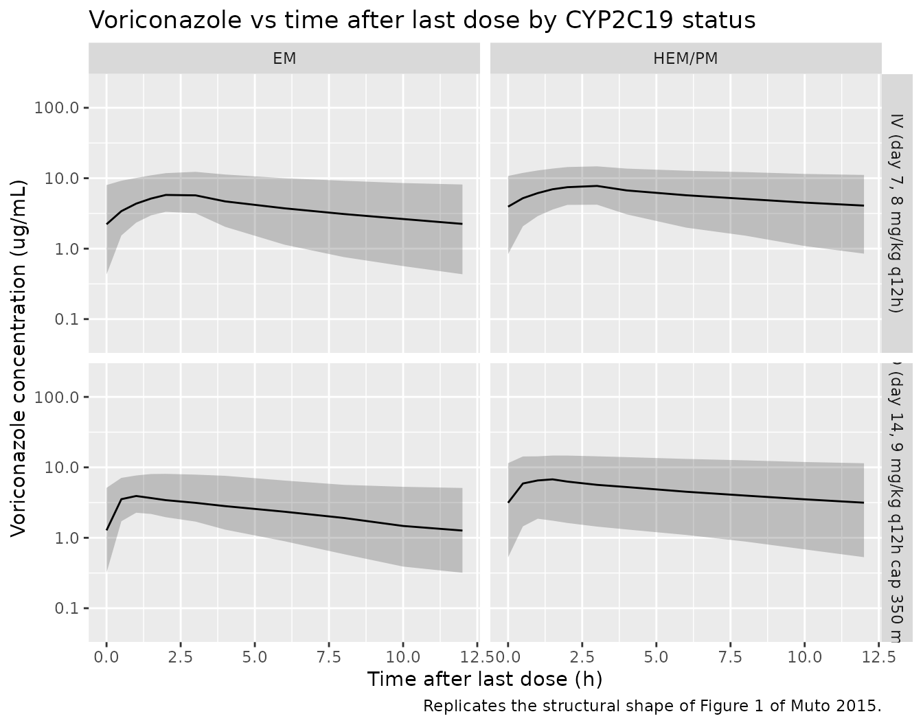
Replicates the structural shape of Figure 1 of Muto 2015: simulated voriconazole concentrations as a function of time after the last steady-state dose, stratified by route (IV day 7, 8 mg/kg q12h vs PO day 14, 9 mg/kg q12h with 350 mg cap) and CYP2C19 status (EM versus HEM+PM).
Figure 2 - Steady-state AUC12 distribution by CYP2C19 status
auc12_iv_subj <- sim |>
  filter(treatment %in% c("Peds 2 to <12 yr", "Adol 1 (<50 kg)"),
         time >= last_dose_iv, time <= last_dose_iv + 12) |>
  group_by(id, cyp_phen) |>
  arrange(time, .by_group = TRUE) |>
  summarise(
    auc12 = sum(diff(time) *
                  (head(Cc, -1) + tail(Cc, -1)) / 2),
    .groups = "drop"
  ) |>
  mutate(cyp_group = if_else(cyp_phen == "EM", "EM", "HEM/PM"))

ggplot(auc12_iv_subj, aes(cyp_group, auc12)) +
  geom_boxplot(width = 0.4, outlier.alpha = 0.4) +
  geom_jitter(width = 0.1, alpha = 0.4, size = 1.2) +
  labs(
    x = "CYP2C19 status",
    y = "AUC12 at 8 mg/kg i.v. q12h (ug.h/mL)",
    title = "Estimated AUC12 by CYP2C19 status (IV day 7)",
    caption = "Replicates the structural shape of Figure 2 (top) of Muto 2015."
  )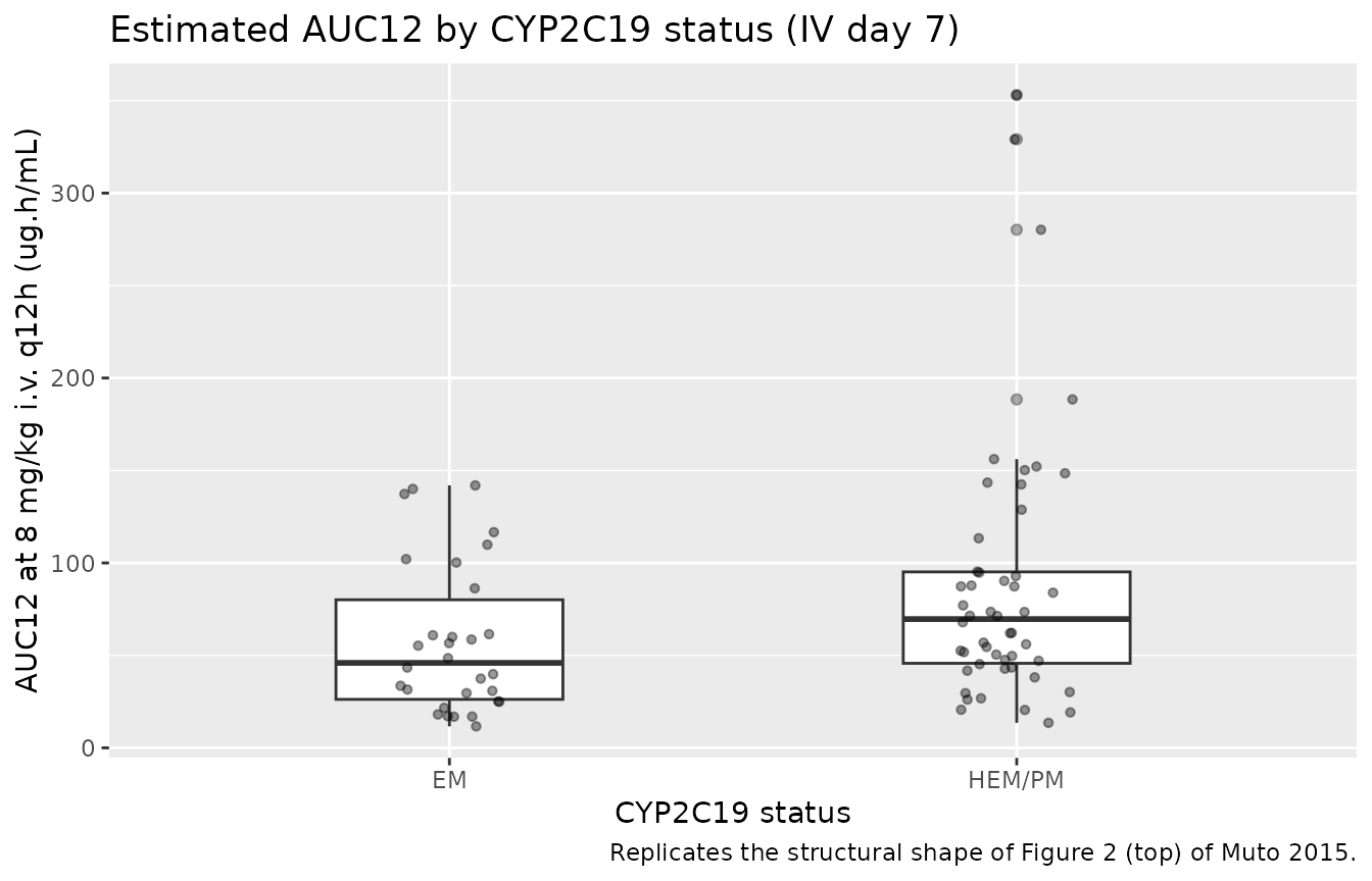
Replicates the structural shape of Figure 2 (top) of Muto 2015: distribution of estimated AUC12 (8 mg/kg i.v. q12h, day 7) by CYP2C19 status.
PKNCA validation
We use PKNCA to compute steady-state PK summaries on the i.v. day-7 dosing interval (t = 144-156 h) and on the oral day-14 dosing interval (t = 312-324 h), stratified by treatment and CYP2C19 status.
conc_iv <- sim |>
  filter(treatment %in% c("Peds 2 to <12 yr", "Adol 1 (<50 kg)"),
         time >= last_dose_iv, time <= last_dose_iv + 12, !is.na(Cc)) |>
  mutate(cyp_group = if_else(cyp_phen == "EM", "EM", "HEM/PM")) |>
  select(id, time, Cc, cyp_group)

# Synthesize a single steady-state dose record per subject for the
# SS NCA interval. The events table uses addl-expansion for the
# i.v. maintenance doses (one row per subject with addl = 11), so the
# explicit dose at t = 144 does not exist as its own row. PKNCA only
# needs one (id, time, amt) record per subject per SS interval.
dose_iv <- events |>
  filter(treatment %in% c("Peds 2 to <12 yr", "Adol 1 (<50 kg)"),
         evid == 1L, cmt == "central", time == 12) |>
  mutate(time = last_dose_iv,
         cyp_group = if_else(cyp_phen == "EM", "EM", "HEM/PM")) |>
  select(id, time, amt, cyp_group)

conc_obj_iv <- PKNCA::PKNCAconc(
  conc_iv, Cc ~ time | cyp_group + id,
  concu = "ug/mL", timeu = "h"
)
dose_obj_iv <- PKNCA::PKNCAdose(
  dose_iv, amt ~ time | cyp_group + id,
  doseu = "mg"
)

intervals_ss <- data.frame(
  start    = last_dose_iv,
  end      = last_dose_iv + 12,
  cmax     = TRUE,
  tmax     = TRUE,
  cmin     = TRUE,
  auclast  = TRUE,
  cav      = TRUE,
  ctrough  = TRUE
)

res_iv <- PKNCA::pk.nca(
  PKNCA::PKNCAdata(conc_obj_iv, dose_obj_iv, intervals = intervals_ss)
)
summary_iv <- as.data.frame(summary(res_iv))
knitr::kable(
  summary_iv,
  caption = "Simulated steady-state NCA on i.v. day 7 (8 mg/kg q12h), stratified by CYP2C19 status."
)| Interval Start | Interval End | cyp_group | N | AUClast (h*ug/mL) | Cmax (ug/mL) | Cmin (ug/mL) | Tmax (h) | Cav (ug/mL) | Ctrough (ug/mL) |
|---|---|---|---|---|---|---|---|---|---|
| 144 | 156 | EM | 30 | 45.3 [83.1] | 6.12 [49.9] | 1.89 [211] | 3.00 [2.00, 3.00] | 3.77 [83.1] | NC |
| 144 | 156 | HEM/PM | 50 | 68.3 [82.6] | 8.12 [57.9] | 3.71 [130] | 3.00 [2.00, 3.00] | 5.69 [82.6] | NC |
conc_po <- sim |>
  filter(treatment %in% c("Peds 2 to <12 yr", "Adol 1 (<50 kg)"),
         time >= last_dose_po, time <= last_dose_po + 12, !is.na(Cc)) |>
  mutate(cyp_group = if_else(cyp_phen == "EM", "EM", "HEM/PM")) |>
  select(id, time, Cc, cyp_group)

# Synthesize a single steady-state dose record per subject for the
# day-14 oral SS interval (the events table uses addl-expansion for
# the oral q12h doses starting at t = 168).
dose_po <- events |>
  filter(treatment %in% c("Peds 2 to <12 yr", "Adol 1 (<50 kg)"),
         evid == 1L, cmt == "depot", time == 168) |>
  mutate(time = last_dose_po,
         cyp_group = if_else(cyp_phen == "EM", "EM", "HEM/PM")) |>
  select(id, time, amt, cyp_group)

conc_obj_po <- PKNCA::PKNCAconc(
  conc_po, Cc ~ time | cyp_group + id,
  concu = "ug/mL", timeu = "h"
)
dose_obj_po <- PKNCA::PKNCAdose(
  dose_po, amt ~ time | cyp_group + id,
  doseu = "mg"
)

intervals_po <- data.frame(
  start    = last_dose_po,
  end      = last_dose_po + 12,
  cmax     = TRUE,
  tmax     = TRUE,
  cmin     = TRUE,
  auclast  = TRUE,
  cav      = TRUE,
  ctrough  = TRUE
)

res_po <- PKNCA::pk.nca(
  PKNCA::PKNCAdata(conc_obj_po, dose_obj_po, intervals = intervals_po)
)
summary_po <- as.data.frame(summary(res_po))
knitr::kable(
  summary_po,
  caption = "Simulated steady-state NCA on p.o. day 14 (9 mg/kg q12h, cap 350 mg), stratified by CYP2C19 status."
)| Interval Start | Interval End | cyp_group | N | AUClast (h*ug/mL) | Cmax (ug/mL) | Cmin (ug/mL) | Tmax (h) | Cav (ug/mL) | Ctrough (ug/mL) |
|---|---|---|---|---|---|---|---|---|---|
| 312 | 324 | EM | 30 | 29.1 [94.5] | 4.20 [65.9] | 1.19 [235] | 1.50 [0.500, 2.00] | 2.42 [94.5] | NC |
| 312 | 324 | HEM/PM | 50 | 48.3 [126] | 5.82 [97.7] | 2.71 [192] | 1.25 [0.500, 4.00] | 4.03 [126] | NC |
Comparison against published Table 5
Muto 2015 Table 5 reports geometric means (CV%) for the pooled Japanese pediatric subjects (n = 18 with oral data) at 8 mg/kg i.v. q12h and 9 mg/kg p.o. q12h (capped at 350 mg). Because Table 5 pools EM and HEM/PM together, the comparison is to the pooled distribution from the two pediatric treatment groups (Peds 2 to <12 yr and Adol 1 (<50 kg)).
pooled_iv <- sim |>
  filter(treatment %in% c("Peds 2 to <12 yr", "Adol 1 (<50 kg)"),
         time >= last_dose_iv, time <= last_dose_iv + 12) |>
  group_by(id) |>
  arrange(time, .by_group = TRUE) |>
  summarise(
    cmax  = max(Cc, na.rm = TRUE),
    cmin  = tail(Cc, 1),
    auc12 = sum(diff(time) *
                  (head(Cc, -1) + tail(Cc, -1)) / 2),
    .groups = "drop"
  )

pooled_po <- sim |>
  filter(treatment %in% c("Peds 2 to <12 yr", "Adol 1 (<50 kg)"),
         time >= last_dose_po, time <= last_dose_po + 12) |>
  group_by(id) |>
  arrange(time, .by_group = TRUE) |>
  summarise(
    cmax  = max(Cc, na.rm = TRUE),
    cmin  = tail(Cc, 1),
    auc12 = sum(diff(time) *
                  (head(Cc, -1) + tail(Cc, -1)) / 2),
    .groups = "drop"
  )

gm <- function(x) exp(mean(log(x[x > 0])))
gcv <- function(x) sqrt(exp(var(log(x[x > 0]))) - 1) * 100

simulated <- bind_rows(
  tibble(
    regimen = "8 mg/kg i.v. q12h",
    metric  = c("AUC12 (ug.h/mL)", "Cmax (ug/mL)", "Cmin (ug/mL)"),
    simulated_gm = c(gm(pooled_iv$auc12), gm(pooled_iv$cmax), gm(pooled_iv$cmin)),
    simulated_cv = c(gcv(pooled_iv$auc12), gcv(pooled_iv$cmax), gcv(pooled_iv$cmin))
  ),
  tibble(
    regimen = "9 mg/kg p.o. q12h (cap 350 mg)",
    metric  = c("AUC12 (ug.h/mL)", "Cmax (ug/mL)", "Cmin (ug/mL)"),
    simulated_gm = c(gm(pooled_po$auc12), gm(pooled_po$cmax), gm(pooled_po$cmin)),
    simulated_cv = c(gcv(pooled_po$auc12), gcv(pooled_po$cmax), gcv(pooled_po$cmin))
  )
)

published <- tibble(
  regimen = c(rep("8 mg/kg i.v. q12h", 3),
              rep("9 mg/kg p.o. q12h (cap 350 mg)", 3)),
  metric  = rep(c("AUC12 (ug.h/mL)", "Cmax (ug/mL)", "Cmin (ug/mL)"), 2),
  published_gm = c(60.3, 7.83, 3.12, 47.8, 6.21, 2.98),
  published_cv = c( 55,   37,    79,    67,   51,   78)
)

simulated |>
  left_join(published, by = c("regimen", "metric")) |>
  mutate(
    simulated_gm = round(simulated_gm, 2),
    simulated_cv = round(simulated_cv, 0)
  ) |>
  knitr::kable(
    caption = "Simulated vs. published (Muto 2015 Table 5) steady-state exposures for the pooled pediatric population. Published values are geometric means with %CV across the published Japanese pediatric cohort (n = 18 for the oral regimen)."
)| regimen | metric | simulated_gm | simulated_cv | published_gm | published_cv |
|---|---|---|---|---|---|
| 8 mg/kg i.v. q12h | AUC12 (ug.h/mL) | 58.68 | 86 | 60.30 | 55 |
| 8 mg/kg i.v. q12h | Cmax (ug/mL) | 7.30 | 57 | 7.83 | 37 |
| 8 mg/kg i.v. q12h | Cmin (ug/mL) | 2.93 | 170 | 3.12 | 79 |
| 9 mg/kg p.o. q12h (cap 350 mg) | AUC12 (ug.h/mL) | 40.02 | 119 | 47.80 | 67 |
| 9 mg/kg p.o. q12h (cap 350 mg) | Cmax (ug/mL) | 5.15 | 88 | 6.21 | 51 |
| 9 mg/kg p.o. q12h (cap 350 mg) | Cmin (ug/mL) | 1.99 | 226 | 2.98 | 78 |
Assumptions and deviations
- Body-weight distribution. Muto 2015 reports a single weight range (11.5-55.2 kg, median 31.5) without per-subject values; the virtual cohort samples weights uniformly within each treatment stratum’s weight band. This is a coarser distribution than the actual cohort, but it preserves the allometric-scaling range and keeps the figures comparable to Table 5 pooled summaries rather than to per-subject exposure points.
-
CYP2C19 distribution. Sampled as 43% EM / 48% HEM /
9% PM to match the cohort frequencies in Table 2 (9 EM, 10 HEM, 2 PM).
HEM and PM are pooled into a single “HEM/PM” stratum throughout the
figures and the i.v. PKNCA comparison, mirroring the paper’s collapsing
of these two genotypes into a single CYP2C19-effect category on
Vmax_inh. The canonical covariate-column register carriesCYP2C19_IMandCYP2C19_PMas separate binary indicators (matching the Zhao 2018 omeprazole register precedent), and the model uses a boolean OR (cyp_hempm = 1 - (1 - CYP2C19_IM) * (1 - CYP2C19_PM)) to recover Muto’s single HEM/PM contrast. - Pooled vs. per-stratum Table 5 comparison. Table 5 reports values pooled across CYP2C19 status for the Japanese subjects who completed each regimen (n = 18 for the oral regimen, n = 21 for the i.v. regimen). The simulated geometric means come from the two pediatric weight strata (Peds 2 to <12 yr and Adol 1 (<50 kg)) pooled across CYP2C19, simulated at the same nominal dose; the Adol 2 stratum is excluded from the pooled comparison because Table 5 reports it only in the within-pool weighted summary, not as the headline number.
- Manly-transformed F1 random effect. Muto 2015 estimates a Manly transformation parameter (theta_BC-F = 0.330) on the eta for F1 to allow a non-Gaussian distribution of individual oral bioavailability after the logit back-transform: ETATR = ((exp(eta))^lambda - 1) / lambda; logit(F1,i) = logit(F1) + ETATR (Table 3 footnote f, Table 4 footnote d). This is encoded literally in the model; downstream simulations of F1 therefore carry a skewed (rather than symmetric) distribution around the typical 64.5% value.
-
Shared Km / Vmax,1 random effect. Muto 2015
enforces 100% correlation between the random effects on Km and Vmax,1 by
sharing a single eta scaled by theta_Vmax,scale = 1.25 (Table 3 footnote
a): Vmax,1,i = Vmax,1 * exp(etalkm_vmax * exp(lvmaxscale)); Km,i = Km *
exp(etalkm_vmax). The shared eta is named
etalkm_vmaxin the model socheckModelConventions()accepts the shared-eta naming pattern without flagging a missing 1-to-1lvmaxpairing. -
Time-dependent Vmax (auto-inhibition). The Appendix
equation Vmax(t) = Vmax,1 * (1 - Vmax_inh * (T-1) / ((T-1) + (T50-1)))
uses
t(time after first dose) starting from zero. At t = 1 h the formula reduces to Vmax = Vmax,1 (the reference). For t in [0, 1) the (T-1) factor in the numerator is negative, giving Vmax > Vmax,1 at very early times after the first dose; this is an artifact of the paper’s parameterisation rather than a physiological prediction. Because PK simulations always start at the first dose (t = 0), this region of the t domain is brief and absorption-limited so the artifact has minimal numerical impact. Implementations that want to avoid the early-time spike could clamp Vmax(t) at Vmax,1 for t < 1, but the model as packaged matches the published equation literally. -
Residual error parameterisation. Muto 2015 fits the
model with log-transformed observations and additive residual error on
the log scale (Methods page 3218). The model is implemented with
Cc ~ lnorm(expSd)andexpSd = 0.239(Table 3); for small residual SDs this is numerically equivalent to a 23.9% proportional error on the linear scale (Table 4 footnote: residual error CV% reported as 23.9%). -
Bayesian priors. Muto 2015 used the NONMEM
NWPRIroutine with normal priors on the fixed-effect parameter vector and inverse Wishart priors on the random-effect covariance, both derived from the Friberg 2012 non-Japanese pediatric + adult model. Because the packaged model carries only the posterior (final) parameter estimates, the prior is not reproduced in the simulation - it influenced the original NONMEM fit but is not needed for the forward-simulation use case of this vignette.