Model and source
- Citation: Zazo H, Lagarejos E, Prado-Velasco M, Sanchez-Herrero S, Serna J, Rueda-Ferreiro A, Martin-Suarez A, Calvo MV, Perez-Blanco JS, Lanao JM. Physiologically-based pharmacokinetic modelling and dosing evaluation of gentamicin in neonates using PhysPK. Front Pharmacol. 2022;13:977372. doi:10.3389/fphar.2022.977372.
- Description (preterm): PBPK (minimal, PhysPK / EcosimPro). Gentamicin in preterm neonates (gestational age 32-37 weeks, postnatal age < 1 week) after a 30-min intravenous infusion. Serum (volume of distribution Vd) is connected to a well-stirred heart chamber perfused at cardiac output, a flow-limited eliminating kidney (elimination flow = TBW * GFR * 0.79, i.e. glomerular filtration net of 21% tubular reabsorption) and a flow-limited rest-of-tissues compartment. Built entirely from literature values with no fitting; between-subject variability is the authors’ log-normal Monte Carlo over GFR, Vd, cardiac output and kidney blood flow. CAUTION: the printed model does not reproduce the paper’s own concentrations. Clearance matches the paper’s Table 4, but simulated serum concentrations at 2 h are 30-40% below the published predictions (Table 4, Figure 2), because the printed serum Vd caps the peak at dose/Vd. The printed serum equation (Eq. 5) is also not mass-conserving and is encoded here in corrected form, and the heart-chamber volume is not reported and is a maintainer assumption. See the vignette Errata before use. Companion model for term neonates: Zazo_2022_gentamicin_term.
- Description (term): PBPK (minimal, PhysPK / EcosimPro). Gentamicin in term neonates (gestational age > 37 weeks, postnatal age < 1 week) after a 30-min intravenous infusion. Serum (volume of distribution Vd) is connected to a well-stirred heart chamber perfused at cardiac output, a flow-limited eliminating kidney (elimination flow = TBW * GFR * 0.79, i.e. glomerular filtration net of 21% tubular reabsorption) and a flow-limited rest-of-tissues compartment. Built entirely from literature values with no fitting; between-subject variability is the authors’ log-normal Monte Carlo over GFR, Vd, cardiac output and kidney blood flow. CAUTION: the printed model does not reproduce the paper’s own concentrations. Clearance matches the paper’s Table 4, but simulated serum concentrations at 2 h are 30-40% below the published predictions (Table 4, Figure 2), because the printed serum Vd caps the peak at dose/Vd. The printed serum equation (Eq. 5) is also not mass-conserving and is encoded here in corrected form, and the heart-chamber volume is not reported and is a maintainer assumption. See the vignette Errata before use. Companion model for preterm neonates: Zazo_2022_gentamicin_preterm.
- Article: https://doi.org/10.3389/fphar.2022.977372 (open access)
Zazo et al. built a minimal physiologically based PK (PBPK) model of gentamicin in neonates in the PhysPK / EcosimPro platform. It has four states: serum, a well-stirred heart chamber perfused by the cardiac output, a flow-limited kidney that eliminates the drug, and a flow-limited “rest of tissues” pool. Every parameter came from the literature; nothing was fitted. Between-subject variability is a log-normal Monte Carlo over body weight, glomerular filtration rate (GFR), serum volume of distribution, cardiac output and kidney blood flow. The authors used one structure with two sets of physiological values, one for preterm and one for term neonates, so the package ships two model files that share this vignette.
Read the Errata section before using these models. Built from the printed equations and tables, the model reproduces the paper’s clearance but not its concentrations. Simulated serum concentrations at 2 h are roughly 30-40% below the paper’s own predictions in Table 4 and Figure 2.
Population
Source paper Table 3: 47 neonates in the first week of life, treated at the University Hospital of Salamanca (Spain) between 1999 and 2003 and monitored by routine TDM, with 91 serum samples taken 2 and 24 h after the start of the infusion.
- Preterm (gestational age 32-37 weeks, n = 31): body weight 1.96 +/- 0.41 kg, postnatal age 3.03 +/- 1.02 days, dose 5.74 +/- 0.80 mg/kg every 48 h.
- Term (gestational age 38-39 weeks, n = 16): body weight 3.09 +/- 0.23 kg, postnatal age 2.94 +/- 0.85 days, dose 6.64 +/- 0.22 mg/kg every 36 h.
These patients validated the model; they were not used to fit it. Sex
distribution is not reported. The same information is available
programmatically, e.g.
readModelDb("Zazo_2022_gentamicin_preterm")()$population.
Source trace
| Equation / parameter | Preterm | Term | Source location |
|---|---|---|---|
d/dt(heart_chamber) |
– | – | Eq. 1 |
d/dt(kidney) |
– | – | Eq. 2 |
qe <- WT * gfr * 0.79 |
– | – | Eq. 3 (21% tubular reabsorption) |
d/dt(other) |
– | – | Eq. 4 |
d/dt(central) |
– | – | Eq. 5, corrected (see Errata) |
cl <- q_kidney * qe / (q_kidney + qe) |
– | – | steady-state clearance of the Eq. 2-3 kidney; compared with Table 4 CL |
lvc (serum Vd, L/kg) |
median of 0.52 +/- 0.16 | median of 0.46 +/- 0.14 | Table 2 |
lgfr (mL/min/kg) |
median of 1.31 +/- 0.53 (= 1.21) | median of 1.72 +/- 0.70 (= 1.59) | Table 2; medians quoted in the Discussion |
lqc (cardiac output, mL/min/kg) |
median of 172 +/- 50.6 | same | Table 2 |
lq_kidney (mL/min/kg) |
median of 9.35, CV 20% | same | Table 1; CV in section 2.1.3 |
lq_other (mL/min/kg) |
217 | same | Table 1 |
lv_kidney (mL) |
0.03 | same | Table 1 |
lv_other (mL) |
0.87 | same | Table 1 |
lkp_kidney |
10.0 | same | Table 1 |
lkp_other |
1.00 | same | Table 1 |
lv_heart_chamber (mL) |
5 | same | not in the paper; assumed by the maintainers |
etalvc |
CV 30.8% | CV 30.4% | Table 2 SD / mean |
etalgfr |
CV 40.5% | CV 40.7% | Table 2 SD / mean (section 2.1.3: 40%) |
etalq_kidney |
CV 20% | same | section 2.1.3 |
etalqc |
CV 29.4% | same | Table 2 SD / mean (section 2.1.3: 24%) |
WT (body weight, kg) |
1.73 +/- 0.35 | 3.56 +/- 0.72 | Table 2 (Monte Carlo); CV 20% in section 2.1.3 |
Each Monte Carlo parameter is reported as an arithmetic mean +/- SD
of a log-normal distribution. The ini() value is the
log-normal median, mean / sqrt(1 + CV^2), and the variance
is omega^2 = log(1 + CV^2). The paper confirms this reading
for GFR: the Discussion quotes the implemented GFR values as 1.21 and
1.59 mL/min/kg. Those are exactly the log-normal medians of Table 2’s
1.31 +/- 0.53 and 1.72 +/- 0.70. The 40% CV in the text would instead
give 1.60 for term neonates.
Structural checks
mod_pre <- readModelDb("Zazo_2022_gentamicin_preterm")
mod_term <- readModelDb("Zazo_2022_gentamicin_term")
typ_pre <- rxode2::zeroRe(mod_pre)
#> ℹ parameter labels from comments will be replaced by 'label()'
typ_term <- rxode2::zeroRe(mod_term)
#> ℹ parameter labels from comments will be replaced by 'label()'
Mass balance of the corrected serum equation
With filtration switched off (lgfr set to a negligible
value), the four states must hold the whole dose forever. Both sides of
the check come from the same solve, so a tight bound applies.
ev_mb <- rxode2::et(amt = 6 * 1.96, dur = 0.5, cmt = "central") |>
  rxode2::et(c(1, 6, 24))
no_elim <- typ_pre |> rxode2::ini(lgfr = log(1e-12))
#> ℹ change initial estimate of `lgfr` to `-27.6310211159285`
mb <- rxode2::rxSolve(no_elim, ev_mb, params = c(WT = 1.96),
                      rtol = 1e-10, atol = 1e-12) |>
  as.data.frame() |>
  mutate(total = central + heart_chamber + kidney + other)
#> ℹ omega/sigma items treated as zero: 'etalvc', 'etalgfr', 'etalq_kidney', 'etalqc'
knitr::kable(mb[, c("time", "central", "heart_chamber", "kidney", "other", "total")],
digits = 6, caption = "Amounts (mg) with elimination switched off; dose 11.76 mg.")| time | central | heart_chamber | kidney | other | total |
|---|---|---|---|---|---|
| 1 | 11.68598 | 0.059982 | 0.003599 | 0.010437 | 11.76 |
| 6 | 11.68598 | 0.059982 | 0.003599 | 0.010437 | 11.76 |
| 24 | 11.68598 | 0.059982 | 0.003599 | 0.010437 | 11.76 |
The serum equation as printed (Eq. 5) has no
-(Qk + Qr) * Cb term. The tissues take up drug from serum
(Eqs. 2 and 4) and return it, but the serum never loses what they take
up, so every pass through a tissue creates drug. Replacing the corrected
line with the printed one shows the consequence:
literal <- typ_pre |>
  rxode2::model(d/dt(central) <- qc * c_heart_chamber + q_kidney * c_kidney / kp_kidney +
                  q_other * c_other / kp_other - qc * Cc)
ev_lit <- rxode2::et(amt = 6 * 1.96, dur = 0.5, cmt = "central") |>
  rxode2::et(c(0.25, 0.5, 1))
lit <- suppressWarnings(rxode2::rxSolve(literal, ev_lit, params = c(WT = 1.96))) |>
  as.data.frame()
#> ℹ omega/sigma items treated as zero: 'etalvc', 'etalgfr', 'etalq_kidney', 'etalqc'
cor <- rxode2::rxSolve(typ_pre, ev_lit, params = c(WT = 1.96)) |> as.data.frame()
#> ℹ omega/sigma items treated as zero: 'etalvc', 'etalgfr', 'etalq_kidney', 'etalqc'
knitr::kable(
  data.frame(time = cor$time, corrected = cor$Cc, printed = lit$Cc),
  digits = 2, format.args = list(big.mark = ","),
  caption = "Typical preterm serum concentration (mg/L), corrected vs. printed Eq. 5."
)| time | corrected | printed |
|---|---|---|
| 0.25 | 5.92 | 7.630600e+02 |
| 0.50 | 11.69 | 6.574143e+05 |
| 1.00 | 11.10 | 4.868502e+11 |
Peak bound
Gentamicin is infused into serum and the tissues are tiny (see Errata), so the serum concentration can never exceed dose / Vd. Table 2 sets Vd at 0.52 L/kg (preterm) and 0.46 L/kg (term), which caps the peak after 6 mg/kg near 11.5 and 13 mg/L. The paper’s Table 4 mean C2h of 17.4 and 15.4 mg/L sit above that cap.
peak_tbl <- bind_rows(lapply(list(list("Preterm", typ_pre, 1.96), list("Term", typ_term, 3.09)), function(g) {
  ev <- rxode2::et(amt = 6 * g[[3]], dur = 0.5, cmt = "central") |> rxode2::et(seq(0, 4, by = 0.05))
  s <- rxode2::rxSolve(g[[2]], ev, params = c(WT = g[[3]])) |> as.data.frame()
  vd <- exp(rxode2::rxode(g[[2]])$theta[["lvc"]]) * g[[3]]
  data.frame(group = g[[1]], cmax = max(s$Cc), bound = 6 * g[[3]] / vd)
}))
#> ℹ omega/sigma items treated as zero: 'etalvc', 'etalgfr', 'etalq_kidney', 'etalqc'
#> ℹ omega/sigma items treated as zero: 'etalvc', 'etalgfr', 'etalq_kidney', 'etalqc'
knitr::kable(peak_tbl, digits = 2,
caption = "Typical-value peak (mg/L) vs. dose / Vd at the Table 3 mean weight.")| group | cmax | bound |
|---|---|---|
| Preterm | 11.69 | 12.07 |
| Term | 13.08 | 13.63 |
Heart-chamber volume sensitivity
The paper does not print the heart-chamber volume Vh; it
is a built-in value of the PhysPK platform. The models carry an assumed
5 mL. Varying it 100-fold shows how little it matters:
vh_tbl <- bind_rows(lapply(c(0.5, 5, 50), function(vh) {
  bind_rows(lapply(list(list("Preterm", typ_pre, 1.96), list("Term", typ_term, 3.09)), function(g) {
    m <- g[[2]] |> rxode2::ini(lv_heart_chamber = log(vh))
    ev <- rxode2::et(amt = 6 * g[[3]], dur = 0.5, cmt = "central") |> rxode2::et(c(2, 24))
    s <- suppressMessages(rxode2::rxSolve(m, ev, params = c(WT = g[[3]]))) |> as.data.frame()
    data.frame(group = g[[1]], vh_mL = vh, C2h = s$Cc[s$time == 2], C24h = s$Cc[s$time == 24])
  }))
}))
#> ℹ change initial estimate of `lv_heart_chamber` to `-0.693147180559945`
#> ℹ change initial estimate of `lv_heart_chamber` to `-0.693147180559945`
#> ℹ change initial estimate of `lv_heart_chamber` to `1.6094379124341`
#> ℹ change initial estimate of `lv_heart_chamber` to `1.6094379124341`
#> ℹ change initial estimate of `lv_heart_chamber` to `3.91202300542815`
#> ℹ change initial estimate of `lv_heart_chamber` to `3.91202300542815`
vh_tbl <- vh_tbl |>
  group_by(group) |>
  mutate(C2h_change_pct = 100 * (C2h / C2h[vh_mL == 5] - 1),
         C24h_change_pct = 100 * (C24h / C24h[vh_mL == 5] - 1)) |>
  ungroup()
knitr::kable(vh_tbl, digits = 2,
caption = "Typical-value C2h and C24h (mg/L) by assumed heart-chamber volume.")| group | vh_mL | C2h | C24h | C2h_change_pct | C24h_change_pct |
|---|---|---|---|---|---|
| Preterm | 0.5 | 10.04 | 1.00 | 0.38 | -0.68 |
| Term | 0.5 | 10.46 | 0.38 | 0.24 | -0.85 |
| Preterm | 5.0 | 10.00 | 1.01 | 0.00 | 0.00 |
| Term | 5.0 | 10.44 | 0.38 | 0.00 | 0.00 |
| Preterm | 50.0 | 9.64 | 1.08 | -3.62 | 6.58 |
| Term | 50.0 | 10.19 | 0.42 | -2.38 | 8.48 |
From 0.5 to 5 mL, C2h and C24h move by under 1%. A 50 mL chamber, close to half of a preterm neonate’s total blood volume, moves C2h by under 5% and C24h by under 15%. Even then, none of the concentration gap in the comparison below is closed.
Virtual cohorts
The paper’s Monte Carlo drew 1,000 virtual patients per group with body weight from Table 2. The cohorts below use 200 per group. The Figure 2 and Table 5 cohorts follow the paper’s Monte Carlo, with weight drawn log-normally from Table 2. The Table 4 clearance comparison uses the observed Table 3 weights, because the paper compares predicted with observed patient clearance (see Errata).
rxode2::rxSetSeed(20221)
set.seed(20221)

draw_lognormal <- function(n, mean, sd) {
  cv <- sd / mean
  mean / sqrt(1 + cv^2) * exp(rnorm(n, 0, sqrt(log(1 + cv^2))))
}

make_cohort <- function(n, wt_mean, wt_sd, dose_mgkg, obs_times, id_offset) {
  subj <- tibble(id = id_offset + seq_len(n), WT = draw_lognormal(n, wt_mean, wt_sd))
  dose <- subj |> mutate(time = 0, evid = 1L, amt = dose_mgkg * WT, dur = 0.5, cmt = "central")
  obs <- subj |>
    tidyr::crossing(time = obs_times) |>
    mutate(evid = 0L, amt = 0, dur = NA_real_, cmt = "central")
  bind_rows(dose, obs) |> arrange(id, time, desc(evid))
}

grid <- seq(0, 72, by = 0.25)
n_arm <- 200L

cohorts <- tibble::tribble(
  ~group,    ~regimen,              ~dose, ~tau, ~wt_mean, ~wt_sd, ~offset,
  "Preterm", "Extended 6 mg/kg q48h",  6,  48,   1.73,     0.35,      0L,
  "Preterm", "Conventional 4 mg/kg q24h", 4, 24, 1.73,     0.35,    200L,
  "Term",    "Extended 6 mg/kg q36h",  6,  36,   3.56,     0.72,    400L,
  "Term",    "Conventional 4 mg/kg q24h", 4, 24, 3.56,     0.72,    600L,
  "Preterm", "Patients (Table 3 weight)", 6, 48, 1.96,     0.41,    800L,
  "Term",    "Patients (Table 3 weight)", 6, 36, 3.09,     0.23,   1000L
)

events <- bind_rows(lapply(seq_len(nrow(cohorts)), function(i) {
  cohorts[i, ] |>
    with(make_cohort(n_arm, wt_mean, wt_sd, dose, grid, offset)) |>
    mutate(group = cohorts$group[i], regimen = cohorts$regimen[i], tau = cohorts$tau[i])
}))
stopifnot(!anyDuplicated(unique(events[, c("id", "time", "evid")])))
Simulation
Each group is solved with its own model file. Only the first dosing interval is used: the paper’s samples (2 and 24 h after the first dose) and its VPC cover the first interval.
sim <- bind_rows(
  rxode2::rxSolve(mod_pre, events = filter(events, group == "Preterm"),
                  keep = c("group", "regimen", "tau", "WT")) |> as.data.frame(),
  rxode2::rxSolve(mod_term, events = filter(events, group == "Term"),
                  keep = c("group", "regimen", "tau", "WT")) |> as.data.frame()
)
#> ℹ parameter labels from comments will be replaced by 'label()'
#> ℹ parameter labels from comments will be replaced by 'label()'
stopifnot(!anyNA(sim$Cc))
Figure 2: visual predictive check
observed <- tibble::tribble(
  ~group,    ~time, ~mean, ~sd,
  "Preterm",     2, 17.7,  4.28,
  "Preterm",    24, 2.92,  0.79,
  "Term",        2, 13.8,  3.08,
  "Term",       24, 1.41,  0.41
)
published_pred <- tibble::tribble(
  ~group,    ~time, ~mean,
  "Preterm",     2, 17.4,
  "Preterm",    24, 2.62,
  "Term",        2, 15.4,
  "Term",       24, 0.89
)

vpc <- sim |>
  filter(grepl("Extended", regimen), time <= tau) |>
  group_by(group, time) |>
  summarise(q05 = quantile(Cc, 0.05), q25 = quantile(Cc, 0.25), q50 = median(Cc),
            q75 = quantile(Cc, 0.75), q95 = quantile(Cc, 0.95), .groups = "drop")

ggplot(vpc, aes(time, q50)) +
  geom_ribbon(aes(ymin = q05, ymax = q95), alpha = 0.2) +
  geom_ribbon(aes(ymin = q25, ymax = q75), alpha = 0.3) +
  geom_line() +
  geom_pointrange(data = observed, aes(y = mean, ymin = mean - sd, ymax = mean + sd),
                  colour = "steelblue") +
  geom_point(data = published_pred, aes(y = mean), shape = 4, size = 3, colour = "firebrick") +
  facet_wrap(~group, scales = "free_x") +
  labs(x = "Time after start of first infusion (h)", y = "Serum gentamicin (mg/L)",
       caption = paste("Replicates Figure 2 of Zazo 2022 (6 mg/kg; 90% and 50% intervals).",
                       "Blue: observed mean +/- SD (Table 3). Red cross: published",
                       "model-predicted mean (Table 4)."))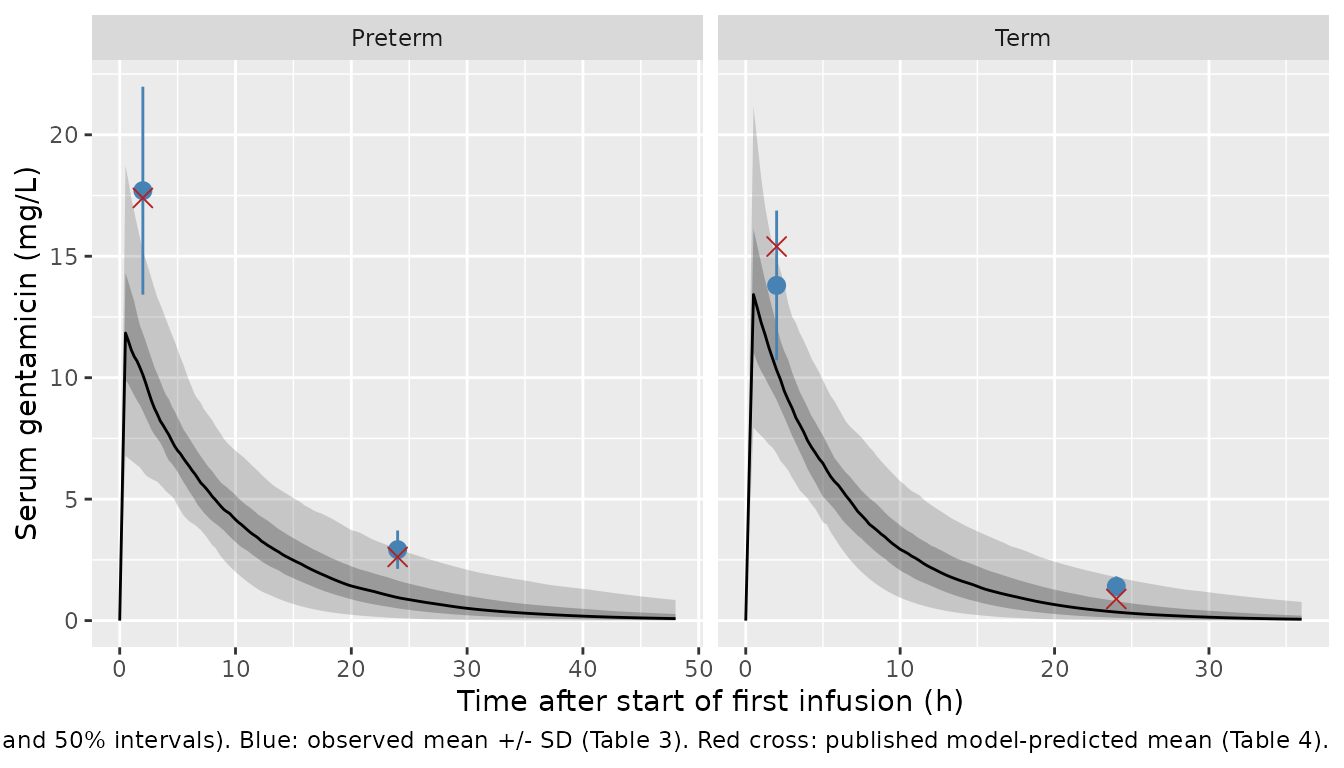
The simulated median peaks near 11-13 mg/L at the end of the infusion. The paper’s Figure 2 median peaks at about 22 mg/L. The observed 2-h concentrations (blue) sit well above the simulated median: the printed model does not reproduce its own VPC.
Table 4: concentrations and clearance
cl_cmp <- sim |>
  filter(regimen == "Patients (Table 3 weight)") |>
  group_by(group) |>
  summarise(
    C2h = mean(Cc[time == 2]),
    C24h = mean(Cc[time == 24]),
    CL = mean(cl[time == 0]),
    .groups = "drop"
  ) |>
  mutate(source = "Simulated (Table 3 weights)")

mc_conc <- sim |>
  filter(grepl("Extended", regimen)) |>
  group_by(group) |>
  summarise(C2h = mean(Cc[time == 2]), C24h = mean(Cc[time == 24]),
            CL = mean(cl[time == 0]), .groups = "drop") |>
  mutate(source = "Simulated (Table 2 weights)")

pub4 <- tibble::tribble(
  ~group,    ~C2h, ~C24h, ~CL,
  "Preterm", 17.4, 2.62,  0.11,
  "Term",    15.4, 0.89,  0.23
) |> mutate(source = "Published prediction (Table 4)")
obs4 <- tibble::tribble(
  ~group,    ~C2h, ~C24h, ~CL,
  "Preterm", 17.7, 2.92,  0.09,
  "Term",    13.8, 1.41,  0.19
) |> mutate(source = "Observed (Table 4)")

bind_rows(cl_cmp, mc_conc, pub4, obs4) |>
  arrange(group, source) |>
  dplyr::rename("Group" = group, "Source" = source, "C2h (mg/L)" = C2h,
                "C24h (mg/L)" = C24h, "CL (L/h)" = CL) |>
knitr::kable(digits = 3, caption = "Mean values, simulated vs. Zazo 2022 Table 4.")| Group | C2h (mg/L) | C24h (mg/L) | CL (L/h) | Source |
|---|---|---|---|---|
| Preterm | 17.700 | 2.920 | 0.090 | Observed (Table 4) |
| Preterm | 17.400 | 2.620 | 0.110 | Published prediction (Table 4) |
| Preterm | 10.325 | 1.184 | 0.093 | Simulated (Table 2 weights) |
| Preterm | 10.181 | 1.242 | 0.110 | Simulated (Table 3 weights) |
| Term | 13.800 | 1.410 | 0.190 | Observed (Table 4) |
| Term | 15.400 | 0.890 | 0.230 | Published prediction (Table 4) |
| Term | 10.611 | 0.565 | 0.250 | Simulated (Table 2 weights) |
| Term | 10.386 | 0.600 | 0.220 | Simulated (Table 3 weights) |
# Clearance reproduces Table 4. CL is an algebraic function of the drawn
# physiology, so the 200-subject mean has a sampling SE near 3%; a
# mis-transcribed GFR, kidney flow or reabsorption factor moves it by far more.
cl_ratio <- cl_cmp$CL / pub4$CL[match(cl_cmp$group, pub4$group)]
stopifnot(all(abs(cl_ratio - 1) < 0.2))
Clearance reproduces Table 4 to within about 10%. That is the model’s
reusable result: a flow-limited kidney with elimination flow
TBW * GFR * 0.79 predicts neonatal gentamicin clearance
from GFR alone. The concentrations do not reproduce. Simulated C2h is
about 40% (preterm) and a third (term) below the published predictions,
and below the observed means. C24h is also below the published
predictions. This is a known deviation of the printed model, not a
simulation artifact (see the peak bound above), so no assertion is
placed on it.
PKNCA validation
sim_nca <- sim |>
  filter(regimen == "Patients (Table 3 weight)", !is.na(Cc)) |>
  select(id, time, Cc, group)
sim_nca <- bind_rows(sim_nca, sim_nca |> distinct(id, group) |> mutate(time = 0, Cc = 0)) |>
  distinct(id, group, time, .keep_all = TRUE) |>
  arrange(id, group, time)

dose_df <- events |>
  filter(evid == 1, regimen == "Patients (Table 3 weight)") |>
  select(id, time, amt, group)

conc_obj <- PKNCA::PKNCAconc(sim_nca, Cc ~ time | group + id)
dose_obj <- PKNCA::PKNCAdose(dose_df, amt ~ time | group + id, route = "intravascular",
                             duration = 0.5)
intervals <- data.frame(start = 0, end = Inf, cmax = TRUE, tmax = TRUE,
                        aucinf.obs = TRUE, half.life = TRUE, cl.obs = TRUE)
nca_res <- PKNCA::pk.nca(PKNCA::PKNCAdata(conc_obj, dose_obj, intervals = intervals))

published_nca <- tibble::tribble(
  ~group,    ~cl.obs,
  "Preterm", 0.11,
  "Term",    0.23
)
cmp <- nlmixr2lib::ncaComparisonTable(
  simulated = nca_res,
  reference = published_nca,
  by = "group",
  units = c(cl.obs = "L/h"),
  tolerance_pct = 20
)
knitr::kable(cmp, caption = "PKNCA clearance (dose / AUC0-inf) vs. Table 4 predicted CL. * differs by >20%.")| NCA parameter | group | Reference | Simulated | % diff |
|---|---|---|---|---|
| CL/F (L/h) | Preterm | 0.11 | 0.104 | -5.1% |
| CL/F (L/h) | Term | 0.23 | 0.211 | -8.1% |
The paper reports no Cmax, AUC or half-life, so clearance is the only NCA quantity with a published counterpart. The full PKNCA summary follows for reference:
| start | end | group | N | cmax | tmax | half.life | aucinf.obs | cl.obs |
|---|---|---|---|---|---|---|---|---|
| 0 | Inf | Preterm | 200 | 11.7 [32.3] | 0.500 [0.500, 0.500] | 7.55 [3.92] | 116 [39.3] | 0.0996 [46.3] |
| 0 | Inf | Term | 200 | 13.1 [30.3] | 0.500 [0.500, 0.500] | 5.08 [2.60] | 89.0 [36.8] | 0.206 [37.6] |
Table 5: probability of target attainment
The target criteria come from source paper section 2.5, with MIC 1 mg/L. The efficacy targets are Cmax/MIC >= 8 and time above MIC >= 60% of the dosing interval. The toxicity targets are Cmin >= 2 mg/L and Cmax >= 25 mg/L. All four are evaluated over the first dosing interval.
pta <- sim |>
  filter(!grepl("Patients", regimen), time <= tau) |>
  group_by(group, regimen, id) |>
  summarise(cmax = max(Cc), cmin = Cc[time == tau[1]],
            tmic = mean(Cc[time < tau[1]] > 1), .groups = "drop") |>
  group_by(group, regimen) |>
  summarise(`Cmax/MIC >= 8` = 100 * mean(cmax >= 8),
            `T>MIC >= 60%` = 100 * mean(tmic >= 0.6),
            `Cmin >= 2 mg/L` = 100 * mean(cmin >= 2),
            `Cmax >= 25 mg/L` = 100 * mean(cmax >= 25),
            .groups = "drop") |>
  mutate(source = "Simulated")
pub5 <- tibble::tribble(
  ~group,    ~regimen,                    ~`Cmax/MIC >= 8`, ~`T>MIC >= 60%`, ~`Cmin >= 2 mg/L`, ~`Cmax >= 25 mg/L`,
  "Preterm", "Conventional 4 mg/kg q24h", 10.8,             87.9,            5.0,               0.0,
  "Preterm", "Extended 6 mg/kg q48h",     99.9,             70.7,            5.9,               6.9,
  "Term",    "Conventional 4 mg/kg q24h", 32.3,             61.2,            0.4,               0.0,
  "Term",    "Extended 6 mg/kg q36h",     99.8,             54.9,            1.8,               6.5
) |> mutate(source = "Published (Table 5)")
bind_rows(pta, pub5) |>
  arrange(group, regimen, source) |>
knitr::kable(digits = 1, caption = "PTA (%) at MIC 1 mg/L, simulated vs. Zazo 2022 Table 5.")| group | regimen | Cmax/MIC >= 8 | T>MIC >= 60% | Cmin >= 2 mg/L | Cmax >= 25 mg/L | source |
|---|---|---|---|---|---|---|
| Preterm | Conventional 4 mg/kg q24h | 10.8 | 87.9 | 5.0 | 0.0 | Published (Table 5) |
| Preterm | Conventional 4 mg/kg q24h | 44.5 | 82.0 | 6.0 | 0.0 | Simulated |
| Preterm | Extended 6 mg/kg q48h | 99.9 | 70.7 | 5.9 | 6.9 | Published (Table 5) |
| Preterm | Extended 6 mg/kg q48h | 90.0 | 30.0 | 0.0 | 2.0 | Simulated |
| Term | Conventional 4 mg/kg q24h | 32.3 | 61.2 | 0.4 | 0.0 | Published (Table 5) |
| Term | Conventional 4 mg/kg q24h | 57.5 | 50.5 | 1.0 | 0.0 | Simulated |
| Term | Extended 6 mg/kg q36h | 99.8 | 54.9 | 1.8 | 6.5 | Published (Table 5) |
| Term | Extended 6 mg/kg q36h | 94.5 | 27.5 | 0.0 | 0.5 | Simulated |
The extended-regimen attainments follow the concentration shortfall. Only neonates with a low drawn Vd reach the 25 mg/L toxicity threshold, a few percent at most against about 7% in Table 5. Time above MIC is also well below the published value. The conventional regimen goes the other way: the model’s Cmax/MIC >= 8 attainment is higher than Table 5’s. Errata item 7 explains why no linear model with log-normally distributed peaks can match Table 5 in full.
Assumptions and deviations
Errata in the source
-
Eq. 5 is not mass-conserving as printed. The serum
equation
Vd dCb/dt = G P(t) + Qh Ch + sum(Qi Ci / Pi) - Qh Cbomits the-sum(Qi) Cboutflow to the kidney and rest of tissues that Eqs. 2 and 4 take up. The models encode the corrected form. PhysPK generates the blood connections itself (section 2.2), so the printed equation is a summary of that code, not the code itself. The correction is the only reading in which the model conserves drug mass (see the mass-balance check above). - Concentrations do not reproduce. With the printed values, simulated C2h is about 30-40% below the paper’s Table 4 predictions and its Figure 2 VPC median. Serum Vd from Table 2 (0.52 / 0.46 L/kg) bounds the peak at dose / Vd, roughly 11.5 / 13 mg/L after 6 mg/kg. The Figure 2 peak of about 22 mg/L implies an apparent volume near 0.27 L/kg. No reading of the organ-volume units closes the gap. Larger tissue volumes only lower the peak further. Halving Vd alone, with clearance held at its Table 4 value, collapses C24h far below the observed values. The maintainers ship the printed values unchanged and do not tune them. The PhysPK model file is not published, and no supplement accompanies the article.
-
Organ-volume units in Table 1. Table 1 labels its
organ volumes “(ml)” with values 0.03 (kidney) and 0.87 (rest of
tissues). Read literally these are far below neonatal physiology, and
they look like L/kg or fractions of body weight. They are encoded as
printed (mL), which leaves the tissues with negligible drug-holding
capacity. Reading them as L or L/kg lowers the simulated peak further,
so the literal reading is also the one closest to the published
concentrations. To test another reading, override
lv_kidney/lv_otherwithrxode2::ini(). - Kidney blood flow. Section 2.1.3 says the kidney flow is in Table 2, but Table 2 has no such row. The models use Table 1’s 9.35 mL/min/kg with the 20% CV stated in section 2.1.3. Table 1’s rest-of-tissues flow (217 mL/min/kg) also exceeds the cardiac output (172 mL/min/kg). In this topology the heart chamber is a parallel recirculation loop, so the tissue flows are not drawn from the cardiac output, and the printed values are used as they are.
- Cardiac-output variability. Section 2.1.3 gives the cardiac-output CV as 24%. Table 2 gives 172 +/- 50.6 mL/min/kg, a CV of 29.4%. The models use Table 2, which is the table of implemented values. For GFR, the Discussion’s 1.21 / 1.59 medians match Table 2’s SD (1.59) better than the text’s 40% CV (1.60). Cardiac output only drives the heart-chamber loop, so the choice has no visible effect on serum concentrations.
- Term dose range. Table 3 prints the term dose range as “6.99 - 6.21” mg/kg, reversed relative to the other rows. It is shown as printed in the population metadata.
- Table 5 peak attainments contradict each other. The model is linear, so a neonate’s peak after 6 mg/kg is 1.5 times its peak after 4 mg/kg. For preterm neonates, Table 5 has 89.2% of 4 mg/kg peaks below 8 mg/L and 99.9% of 6 mg/kg peaks at or above 8 mg/L. That puts 4 mg/kg peaks at or above 5.3 mg/L in 99.9% of neonates. So 89% of the 4 mg/kg peaks must lie between 5.3 and 8 mg/L. Yet 6.9% of 6 mg/kg peaks reach 25 mg/L, which needs a 4 mg/kg peak of 16.7 mg/L or more. A log-normal peak that fits the first two figures puts essentially no neonate above 16.7 mg/L. No single log-normal peak distribution satisfies all three figures, so the comparison above is descriptive only.
Non-paper-derived values
-
Heart-chamber volume
Vh= 5 mL is assumed by the maintainers. The paper usesVhin Eq. 1 but never gives a value (it is a PhysPK built-in). The sensitivity table above shows that a 0.5-50 mL range leaves the conclusions unchanged. -
No residual error. The paper’s Monte Carlo varied
physiology only, so
propSdis held at zero.
Other modelling choices
- The 30-min infusion pulse
G P(t)of Eq. 5 is supplied by the dosing record (dur = 0.5,cmt = "central") rather than written into the ODE. - Body weight is a covariate (
WT), not a random effect. The paper’s log-normal TBW draw (Table 2, CV 20%) is reproduced in the virtual cohort. - The paper notes that the Monte Carlo draws were uncorrelated; the models carry a diagonal OMEGA.
- The PTA comparison uses the first dosing interval. The paper does not say whether Table 5 used the first interval or steady state.
- The paper also estimated GFR with the PhysPK estimation module (1.176 +/- 0.037 and 1.324 +/- 0.054 mL/min/kg). Those values were a software check and are not part of the model.