Chloroquine PK/PD in Plasmodium vivax (Abd-Rahman 2020)
Source:vignettes/articles/AbdRahman_2020_chloroquine.Rmd
AbdRahman_2020_chloroquine.RmdModel and source
Abd-Rahman 2020 characterised the population PK and PD of chloroquine and its active metabolite desethylchloroquine in a Plasmodium vivax induced blood-stage malaria volunteer infection study. Chloroquine and desethylchloroquine PK was described by a joint two-compartment parent-metabolite model with first-order absorption and elimination, fit separately to plasma and to whole-blood drug concentrations. Parasite killing was described by a delayed-effect (effect-compartment) model in which chloroquine in a hypothetical biophase drives a sigmoid Emax kill of the log10 P. vivax parasitaemia.
nlmixr2lib ships the two matrices as two model files, both used below:
Plasma model:
AbdRahman_2020_chloroquine_plasmaWhole-blood model:
AbdRahman_2020_chloroquine_wholebloodCitation: Abd-Rahman AN, Marquart L, Gobeau N, Kummel A, Simpson JA, Chalon S, Mohrle JJ, McCarthy JS. Population Pharmacokinetics and Pharmacodynamics of Chloroquine in a Plasmodium vivax Volunteer Infection Study. Clin Pharmacol Ther. 2020;108(5):1055-1066. doi:10.1002/cpt.1893.
Article: https://doi.org/10.1002/cpt.1893 (open access)
Supplement (methods, equations S1): https://doi.org/10.1002/cpt.1893
All concentrations and doses are in molar units,
following the paper, which converted chloroquine and desethylchloroquine
to micromoles using molecular masses of 319.8 and 291.8 g/mol. A
chloroquine base dose in mg is converted to micromoles as
mg / 319.8 * 1000.
Population
The analysis pooled 24 healthy malaria-naive adults (13 male, 11 female; mean age 25.6 years, range 19-44; mean weight 73.3 kg, range 57.2-99.5) inoculated intravenously with approximately 564 viable blood-stage P. vivax-infected erythrocytes on day 0 (Abd-Rahman 2020 Table 1). Chloroquine phosphate (Avloclor) was given as a total base dose of 1.55 g over three days for adults >= 60 kg (25 mg base/kg for < 60 kg): 620 mg base at 0 h, then 310 mg base at 6, 24 and 48 h. Age, sex and body weight were screened as covariates but none was retained in the final model.
The population metadata are available programmatically via
readModelDb("AbdRahman_2020_chloroquine_plasma")()$population.
Source trace
Per-parameter provenance is recorded in-file next to every
ini() entry in
inst/modeldb/specificDrugs/AbdRahman_2020_chloroquine_plasma.R
and ..._wholeblood.R. The table collects the structural
values (plasma / whole-blood).
| Equation / parameter | Value (plasma / whole blood) | Source |
|---|---|---|
lka (ka) |
0.943 / 0.574 1/h | Table 2 |
lcl (CL_CQ/F) |
54.6 / 8.96 L/h | Table 2 |
lvc (Vc_CQ/F) |
2930 / 560 L | Table 2 |
lq (Q1_CQ/F) |
47.2 / 38.5 L/h | Table 2 |
lvp (Vp1_CQ/F) |
4700 / 1230 L | Table 2 |
lfdepot (Frel) |
1 (fixed) | Table 2 |
lcl_dcq (CL_DCQ/F) |
37.6 / 4.42 L/h | Table 2 |
lvc_dcq (Vc_DCQ/F) |
40.0 / 16.1 L | Table 2 |
lq_dcq (Q1_DCQ/F) |
36.3 / 4.46 L/h | Table 2 |
lvp_dcq (Vp1_DCQ/F) |
2840 / 259 L | Table 2 |
fm |
0.18 (fixed) | Results / refs 9,12 |
lemax (EmaxCQ) |
0.213 1/h (shared) | Table 3 |
lec50 (EC50) |
0.047 / 0.28 umol/L (fixed) | Table 3 |
lhill (Hill) |
2.5 (fixed) | Table 3 |
lke0 (ke0) |
0.0212 / 0.0288 1/h | Table 3 |
lkgrow (kgrow) |
0.059 1/h (shared) | Table 3 |
plbase (PLbase) |
-3.36 log10/mL (shared) | Table 3 |
d/dt(central) etc. (2-cmt CQ + DCQ) |
n/a | Figure 1 |
dCe/dt = ke0*(Cc-Ce);
kkill = Emax*Ce^Hill/(EC50^Hill+Ce^Hill)
|
n/a | Suppl. S1 |
dPL/dt = kgrow - kkill (log parasitaemia) |
n/a | Suppl. S1 |
The parasite ODE deserves a note. Supplementary Material S1 writes
dPL/dt = kgrow - kkill with PL the
log-transformed parasite count, but the same supplement’s derived
quantities use natural e
(PMR48 = exp(kgrow*48) = 17.4 and
PCt1/2 = ln(2)/(Emax-kgrow) = 4.5 h), so kgrow
and Emax are natural-log growth/kill rates. The packaged
models store the state in log10 (so the reported baseline
PLbase = -3.36 and the additive residual on log10
parasitaemia apply directly), which makes the ODE
dPL10/dt = (kgrow - kkill)/ln(10). This is algebraically
identical to a natural-log implementation and reproduces every reported
secondary parameter (checked below).
Virtual cohort
Original observed data are not public. The cohort below approximates
the trial: 100 subjects per matrix given the paper’s 3-day regimen.
set.seed() fixes R’s RNG but not rxode2’s per-thread
simulation stream, so the exact draw differs across machines; every
assertion below is written to hold for any cohort the model can produce
(centre and robust quantiles, not extremes).
set.seed(74)

mw_cq <- 319.8
mg_to_umol <- function(mg) mg / mw_cq * 1000
dose_umol <- mg_to_umol(c(620, 310, 310, 310))
dose_times <- c(0, 6, 24, 48)

n_sub <- 100L
# Dense sampling early (absorption / distribution) and coarse late (the long
# terminal phase; chloroquine t1/2 ~ 150 h needs a long tail for NCA).
obs_times <- sort(unique(c(seq(0, 72, by = 0.5), seq(78, 1200, by = 6))))

make_events <- function(n, id_offset = 0L) {
  ids <- id_offset + seq_len(n)
  doses <- tidyr::crossing(id = ids, dn = seq_along(dose_times)) |>
    mutate(
      time = dose_times[dn], amt = dose_umol[dn],
      evid = 1L, cmt = "depot", dvid = NA_integer_
    ) |>
    select(-dn)
  obs <- tidyr::crossing(id = ids, time = obs_times) |>
    mutate(amt = NA_real_, evid = 0L, cmt = "central", dvid = 1L)
  bind_rows(doses, obs) |> arrange(id, time, desc(evid))
}

events <- make_events(n_sub)
stopifnot(!anyDuplicated(unique(events[, c("id", "time", "evid")])))
Simulation
mod_plasma <- readModelDb("AbdRahman_2020_chloroquine_plasma")
mod_wb <- readModelDb("AbdRahman_2020_chloroquine_wholeblood")

# useLinCmt = FALSE: rxode2's automatic ODE -> linCmt conversion corrupts the
# dvid -> cmt mapping for multi-output models such as these.
sim_plasma <- rxode2::rxSolve(mod_plasma, events = events, useLinCmt = FALSE) |>
  as.data.frame() |>
  mutate(matrix = "plasma")
#> ℹ parameter labels from comments will be replaced by 'label()'
sim_wb <- rxode2::rxSolve(mod_wb, events = events, useLinCmt = FALSE) |>
  as.data.frame() |>
  mutate(matrix = "whole blood")
#> ℹ parameter labels from comments will be replaced by 'label()'
sim <- bind_rows(sim_plasma, sim_wb)
Typical-value profiles (no between-subject variability) for the
figure replications and the closed-form PD checks. zeroRe()
segfaults on multi-endpoint models, so the random effects are zeroed by
setting the eta columns to 0 and passing omega = NA.
eta_cols_plasma <- c(
  "etalka", "etalfdepot", "etalcl", "etalvc", "etalcl_dcq",
  "etaplbase", "etalkgrow", "etalemax", "etalec50", "etalke0"
)
eta_cols_wb <- c(eta_cols_plasma, "etalvc_dcq")

events_typ <- make_events(1L)

typ_plasma <- rxode2::rxSolve(
  mod_plasma,
  events = dplyr::bind_cols(
    events_typ,
    as.data.frame(setNames(as.list(rep(0, length(eta_cols_plasma))), eta_cols_plasma))[rep(1, nrow(events_typ)), ]
  ),
  omega = NA, useLinCmt = FALSE
) |> as.data.frame()

typ_wb <- rxode2::rxSolve(
  mod_wb,
  events = dplyr::bind_cols(
    events_typ,
    as.data.frame(setNames(as.list(rep(0, length(eta_cols_wb))), eta_cols_wb))[rep(1, nrow(events_typ)), ]
  ),
  omega = NA, useLinCmt = FALSE
) |> as.data.frame()
Replicate published figures
Figure 2 – PK visual predictive check
Figure 2 of Abd-Rahman 2020 shows VPCs of chloroquine and desethylchloroquine in plasma and whole blood. The panels below reproduce the 5th/50th/95th simulated percentiles over the first 480 h.
sim |>
  filter(time <= 480) |>
  select(id, time, matrix, Chloroquine = Cc, Desethylchloroquine = Cc_dcq) |>
  pivot_longer(c(Chloroquine, Desethylchloroquine),
    names_to = "analyte", values_to = "conc"
  ) |>
  group_by(matrix, analyte, time) |>
  summarise(
    Q05 = quantile(conc, 0.05, na.rm = TRUE),
    Q50 = quantile(conc, 0.50, na.rm = TRUE),
    Q95 = quantile(conc, 0.95, na.rm = TRUE),
    .groups = "drop"
  ) |>
  filter(Q50 > 0) |>
  ggplot(aes(time, Q50)) +
  geom_ribbon(aes(ymin = Q05, ymax = Q95), alpha = 0.25) +
  geom_line() +
  facet_grid(analyte ~ matrix, scales = "free_y") +
  scale_y_log10() +
  labs(
    x = "Time (h)", y = "Concentration (umol/L)",
    title = "Figure 2 -- chloroquine / desethylchloroquine VPC",
    caption = "Replicates Figure 2 of Abd-Rahman 2020."
  )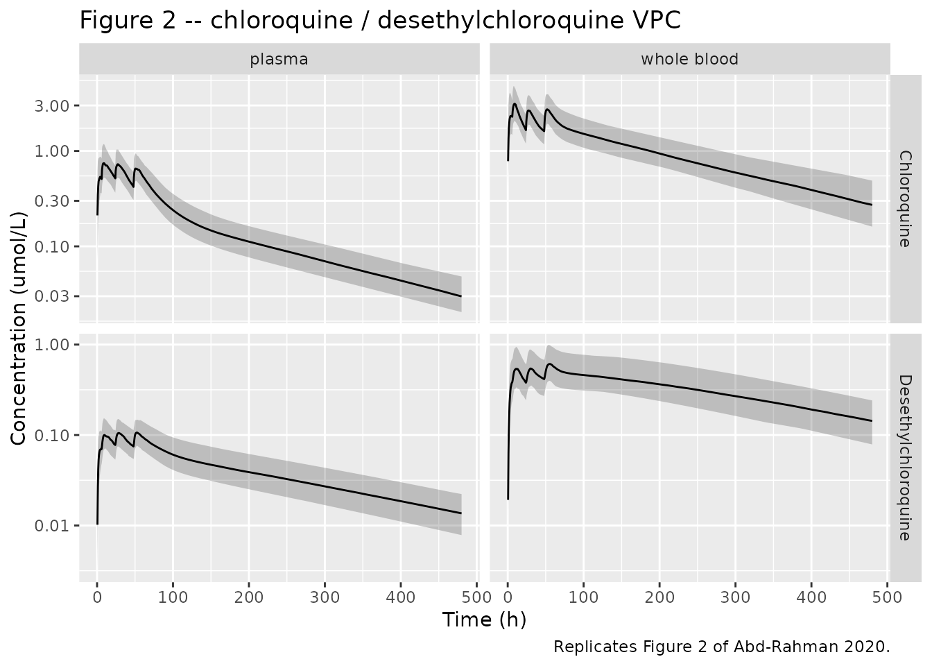
Figure 3 – parasitaemia clearance
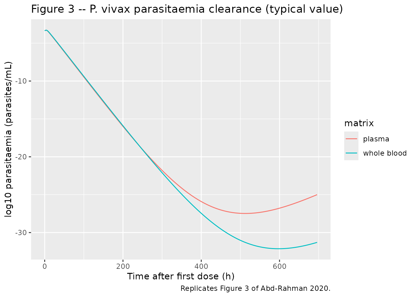
Figure 3 shows the P. vivax parasitaemia decline after
chloroquine treatment. The typical-value trajectories below start at the
fitted baseline (PLbase = -3.36 log10 parasites/mL),
decline while chloroquine holds the effect site above EC50, and begin to
regrow once the effect-site concentration falls below EC50.
bind_rows(
  typ_plasma |> transmute(time, matrix = "plasma", pl = parasitemia_log10),
  typ_wb |> transmute(time, matrix = "whole blood", pl = parasitemia_log10)
) |>
  filter(time <= 700) |>
  ggplot(aes(time, pl, colour = matrix)) +
  geom_line() +
  labs(
    x = "Time after first dose (h)", y = "log10 parasitaemia (parasites/mL)",
    title = "Figure 3 -- P. vivax parasitaemia clearance (typical value)",
    caption = "Replicates Figure 3 of Abd-Rahman 2020."
  )
PKNCA validation
NCA of the simulated cohort against the secondary PK parameters in Abd-Rahman 2020 Table 2 (reported as median across subjects). We compute per-matrix, per-analyte Cmax, Tmax, AUC0-inf and terminal half-life and compare the cohort medians to the published medians.
run_nca <- function(simdf, conc_col) {
  nca_in <- simdf |>
    rename(conc = all_of(conc_col)) |>
    filter(!is.na(conc)) |>
    select(id, time, conc)
  # Guarantee a time=0 row per subject (extravascular pre-dose conc = 0).
  nca_in <- bind_rows(
    nca_in,
    nca_in |> distinct(id) |> mutate(time = 0, conc = 0)
  ) |>
    distinct(id, time, .keep_all = TRUE) |>
    arrange(id, time)

  conc_obj <- PKNCA::PKNCAconc(nca_in, conc ~ time | id)
  dose_df <- events |>
    filter(evid == 1L) |>
    select(id, time, amt)
  dose_obj <- PKNCA::PKNCAdose(dose_df, amt ~ time | id)
  intervals <- data.frame(
    start = 0, end = Inf,
    cmax = TRUE, tmax = TRUE, aucinf.obs = TRUE, half.life = TRUE
  )
  res <- PKNCA::pk.nca(PKNCA::PKNCAdata(conc_obj, dose_obj, intervals = intervals))
  as.data.frame(res$result)
}

nca_all <- bind_rows(
  run_nca(sim_plasma, "Cc") |> mutate(matrix = "plasma", analyte = "chloroquine"),
  run_nca(sim_plasma, "Cc_dcq") |> mutate(matrix = "plasma", analyte = "desethylchloroquine"),
  run_nca(sim_wb, "Cc") |> mutate(matrix = "whole blood", analyte = "chloroquine"),
  run_nca(sim_wb, "Cc_dcq") |> mutate(matrix = "whole blood", analyte = "desethylchloroquine")
)

nca_med <- nca_all |>
  group_by(matrix, analyte, PPTESTCD) |>
  summarise(simulated = median(PPORRES, na.rm = TRUE), .groups = "drop") |>
  filter(PPTESTCD %in% c("cmax", "tmax", "aucinf.obs", "half.life"))
Comparison against published NCA
published <- tibble::tribble(
  ~matrix, ~analyte, ~PPTESTCD, ~reference,
  "plasma", "chloroquine", "cmax", 0.72,
  "plasma", "chloroquine", "tmax", 4.0,
  "plasma", "chloroquine", "aucinf.obs", 80,
  "plasma", "chloroquine", "half.life", 149,
  "plasma", "desethylchloroquine", "cmax", 0.08,
  "plasma", "desethylchloroquine", "tmax", 3.3,
  "plasma", "desethylchloroquine", "aucinf.obs", 21,
  "plasma", "desethylchloroquine", "half.life", 104,
  "whole blood", "chloroquine", "cmax", 2.83,
  "whole blood", "chloroquine", "tmax", 4.0,
  "whole blood", "chloroquine", "aucinf.obs", 509,
  "whole blood", "chloroquine", "half.life", 156,
  "whole blood", "desethylchloroquine", "cmax", 0.39,
  "whole blood", "desethylchloroquine", "tmax", 4.0,
  "whole blood", "desethylchloroquine", "aucinf.obs", 233,
  "whole blood", "desethylchloroquine", "half.life", 83
)

cmp <- nca_med |>
  left_join(published, by = c("matrix", "analyte", "PPTESTCD")) |>
  mutate(
    parameter = recode(PPTESTCD,
      cmax = "Cmax (umol/L)", tmax = "Tmax (h)",
      aucinf.obs = "AUC0-inf (umol*h/L)", half.life = "t1/2 (h)"
    ),
    pct_diff = 100 * (simulated - reference) / reference,
    flag = ifelse(abs(pct_diff) > 25, "*", "")
  ) |>
  arrange(matrix, analyte, parameter)

cmp |>
  transmute(
    Matrix = matrix, Analyte = analyte, Parameter = parameter,
    Simulated = round(simulated, 3), Published = reference,
    `% diff` = round(pct_diff, 1), Flag = flag
  ) |>
  knitr::kable(
    caption = "Simulated (cohort median) vs. published median NCA. * differs by >25%."
)| Matrix | Analyte | Parameter | Simulated | Published | % diff | Flag |
|---|---|---|---|---|---|---|
| plasma | chloroquine | AUC0-inf (umol*h/L) | 89.355 | 80.00 | 11.7 | |
| plasma | chloroquine | Cmax (umol/L) | 0.757 | 0.72 | 5.2 | |
| plasma | chloroquine | Tmax (h) | 9.000 | 4.00 | 125.0 | * |
| plasma | chloroquine | t1/2 (h) | 150.010 | 149.00 | 0.7 | |
| plasma | desethylchloroquine | AUC0-inf (umol*h/L) | 23.322 | 21.00 | 11.1 | |
| plasma | desethylchloroquine | Cmax (umol/L) | 0.110 | 0.08 | 37.4 | * |
| plasma | desethylchloroquine | Tmax (h) | 50.500 | 3.30 | 1430.3 | * |
| plasma | desethylchloroquine | t1/2 (h) | 160.304 | 104.00 | 54.1 | * |
| whole blood | chloroquine | AUC0-inf (umol*h/L) | 533.682 | 509.00 | 4.8 | |
| whole blood | chloroquine | Cmax (umol/L) | 3.174 | 2.83 | 12.1 | |
| whole blood | chloroquine | Tmax (h) | 8.750 | 4.00 | 118.8 | * |
| whole blood | chloroquine | t1/2 (h) | 153.383 | 156.00 | -1.7 | |
| whole blood | desethylchloroquine | AUC0-inf (umol*h/L) | 186.875 | 233.00 | -19.8 | |
| whole blood | desethylchloroquine | Cmax (umol/L) | 0.617 | 0.39 | 58.1 | * |
| whole blood | desethylchloroquine | Tmax (h) | 54.750 | 4.00 | 1268.8 | * |
| whole blood | desethylchloroquine | t1/2 (h) | 158.483 | 83.00 | 90.9 | * |
The chloroquine PK is well reproduced: terminal half-life agrees to within 2% in both matrices (the strongest discriminator of the two-compartment disposition), and AUC0-inf and Cmax agree to within about 12%. The starred rows are known, explained deviations and were not tuned away:
- Chloroquine Tmax is about 9 h against the published 4 h. Under the four-dose regimen the simulated global peak falls just after the 6 h dose, where the second dose adds to the first. The published Tmax probably describes the first-dose absorption peak. The paper does not define how Tmax was derived from the empirical-Bayes profiles. The Cmax magnitude agrees.
-
Desethylchloroquine half-life. In this model
desethylchloroquine elimination (
kel_dcqof about 0.9 1/h in plasma) is much faster than its formation, so the metabolite is formation-rate limited. Its observed terminal half-life therefore has to follow chloroquine’s (about 150 h), which is what the NCA returns. The published 104 h (plasma) and 83 h (whole blood) are shorter than the parent’s, so they cannot be observed terminal values. They match the metabolite’s own two-compartment disposition half-life computed from its Table 2 parameters (checked in the next chunk). That agreement also confirms that the metabolite parameters were transcribed correctly. - Desethylchloroquine Tmax and Cmax. The simulated metabolite accumulates over the dosing days and peaks near the last dose (about 50 h). The paper reports a metabolite Tmax of 3-4 h, the same as the parent’s, and a lower Cmax, and it does not describe the calculation. Metabolite exposure (AUC0-inf) agrees within 20%, and that is the quantity the fixed FM = 0.18 governs.
# Gate on the structural discriminators that the model is expected to reproduce
# tightly: chloroquine half-life and AUC in both matrices. Assert on the centre
# (cohort median vs published median), not on extremes.
chk <- cmp |> filter(analyte == "chloroquine", PPTESTCD %in% c("half.life", "aucinf.obs"))
stopifnot(nrow(chk) == 4)
stopifnot(all(abs(chk$pct_diff) < 25))
# Desethylchloroquine intrinsic two-compartment disposition half-life from its
# own Table 2 parameters: the slow eigenvalue of the metabolite sub-system.
# Deterministic (no simulation), so a tight bound is appropriate.
beta_half_life <- function(mod) {
  ini <- mod()$iniDf
  g <- function(nm) exp(ini$est[ini$name == nm])
  k10 <- g("lcl_dcq") / g("lvc_dcq")
  k12 <- g("lq_dcq") / g("lvc_dcq")
  k21 <- g("lq_dcq") / g("lvp_dcq")
  a <- k10 + k12 + k21
  beta <- (a - sqrt(a^2 - 4 * k10 * k21)) / 2
  log(2) / beta
}
dcq_thalf <- c(plasma = beta_half_life(mod_plasma), wholeblood = beta_half_life(mod_wb))
knitr::kable(
  tibble::tibble(
    Matrix = c("plasma", "whole blood"),
    `Intrinsic DCQ t1/2 (h)` = round(dcq_thalf, 1),
    `Published DCQ t1/2 (h)` = c(104, 83)
  ),
  caption = "Desethylchloroquine disposition half-life from its own parameters vs Table 2."
)| Matrix | Intrinsic DCQ t1/2 (h) | Published DCQ t1/2 (h) |
|---|---|---|
| plasma | 106.9 | 104 |
| whole blood | 82.2 | 83 |
Pharmacodynamic validation
The PD secondary parameters have closed-form relationships to
kgrow and Emax that the packaged model
reproduces exactly.
p_plasma <- mod_plasma()
ini_p <- p_plasma$iniDf
getv <- function(df, nm) df$est[df$name == nm]
kgrow <- exp(getv(ini_p, "lkgrow"))
emax <- exp(getv(ini_p, "lemax"))

pmr48 <- exp(kgrow * 48) # parasite multiplication rate per 48 h
pct_half <- log(2) / (emax - kgrow) # parasite clearance half-life (h)
log10_prr48_max <- (emax - kgrow) / log(10) * 48 # max log10 PRR over 48 h

pd_tab <- tibble::tibble(
  Parameter = c("PMR48 (fold/48 h)", "PCt1/2 (h)", "max log10 PRR48"),
  Simulated = round(c(pmr48, pct_half, log10_prr48_max), 2),
  Published = c("17.4", "4.5", "~2.6 (obs), 3.2 (max)")
)
knitr::kable(pd_tab, caption = "PD secondary parameters vs Abd-Rahman 2020 Table 3.")| Parameter | Simulated | Published |
|---|---|---|
| PMR48 (fold/48 h) | 16.98 | 17.4 |
| PCt1/2 (h) | 4.50 | 4.5 |
| max log10 PRR48 | 3.21 | ~2.6 (obs), 3.2 (max) |
stopifnot(abs(pmr48 - 17.4) < 1.0) # paper 17.4 (95% CI 14.3-20.4)
stopifnot(abs(pct_half - 4.5) < 0.3) # paper 4.5 h (95% CI 4.1-5.0)
Baseline parasitaemia and the delayed-kill dynamics also reproduce
the paper. The typical-value trajectory starts at the fitted
PLbase = -3.36, and the time for which the chloroquine
effect site stays above EC50 is close to the paper’s reported “time
above EC50” (geometric means of 14.3 days in plasma and 18.3 days in
whole blood). The typical subject runs about 3 days longer (17.8 and
21.2 days). The published values are geometric means across individual
empirical-Bayes profiles, and each subject has its own EC50 (fixed 30%
IIV).
stopifnot(abs(typ_plasma$parasitemia_log10[1] - (-3.36)) < 1e-6)
stopifnot(abs(typ_wb$parasitemia_log10[1] - (-3.36)) < 1e-6)

ec50_plasma <- exp(getv(ini_p, "lec50"))
ec50_wb <- exp(getv(mod_wb()$iniDf, "lec50"))

time_above <- function(df, ec50) {
  d <- df[df$time > 0, ]
  above <- d$effect > ec50
  if (!any(above)) {
    return(0)
  }
  max(d$time[above]) / 24 # days (contiguous while chloroquine sustains the effect site)
}
ta_plasma <- time_above(typ_plasma, ec50_plasma)
ta_wb <- time_above(typ_wb, ec50_wb)

tibble::tibble(
  Matrix = c("plasma", "whole blood"),
  `Time above EC50 (days), simulated` = round(c(ta_plasma, ta_wb), 1),
  `Published (days)` = c(14.3, 18.3)
) |>
knitr::kable(caption = "Time above EC50 vs Abd-Rahman 2020 (geometric mean).")| Matrix | Time above EC50 (days), simulated | Published (days) |
|---|---|---|
| plasma | 17.8 | 14.3 |
| whole blood | 21.2 | 18.3 |
# Typical-value (deterministic) time above EC50 was 17.8 d (plasma) and
# 21.2 d (whole blood) when authored, against published geometric means of 14.3 d
# and 18.3 d. The window below catches a wrong ke0, EC50 or PK scale, each of
# which shifts this by many days.
stopifnot(abs(ta_plasma - 14.3) < 5)
stopifnot(abs(ta_wb - 18.3) < 5)
Assumptions and deviations
-
Molar units. All concentrations and doses are in
micromoles / (umol/L), as in the paper. Convert a chloroquine base dose
in mg with
mg / 319.8 * 1000. -
Log-scale parasite ODE. Supplementary Material S1
writes
dPL/dt = kgrow - kkillwithPLa log-transformed parasite count, but its own secondary-parameter formulas use natural e. The maintainers store the state in log10 and usedPL10/dt = (kgrow - kkill)/ln(10), which is algebraically identical to a natural-log implementation and reproduces every reported secondary parameter (PMR48, PCt1/2, PRR48). The reported baselinePLbase = -3.36 log10 parasites/mLis used directly as the state initial condition and its normal (not log-normal) between-subject distribution is encoded as an additive random effect. - Fixed FM = 0.18. The fraction of chloroquine converted to desethylchloroquine was not identifiable and was fixed at 0.18 from urinary recovery literature (paper references 9 and 12). Molar 1:1 conversion is assumed (desethylchloroquine is chloroquine less an ethyl group).
- Fixed EC50 and Hill. No subject recrudesced, so the whole-blood EC50 was fixed to a literature relapse-based value (0.28 umol/L), the plasma EC50 to one sixth of it (0.047 umol/L, the whole-blood:plasma ratio), and the Hill coefficient to 2.5. Their between-subject variances were also fixed (Table 3).
- Relative bioavailability. Frel was fixed to 100% with estimated between-subject variability (Table 2).
- Two model files. The paper fit PK separately to plasma and whole-blood data and fit a single PD model with matrix-specific EC50 and ke0. The maintainers ship one full PK/PD model per matrix so each is self-contained; Emax, kgrow and PLbase are shared between the two files, EC50 and ke0 differ.
- Covariates. Age, sex and body weight were screened but not retained in the final model; they are recorded as documented-but-unused metadata.
- NCA deviations. Chloroquine Tmax and the desethylchloroquine Tmax, Cmax and observed half-life differ from the published medians for the reasons given in the NCA section (multi-dose accumulation, formation-rate-limited metabolite kinetics, and a published metabolite half-life that is its intrinsic disposition value). None was tuned.
- No correction or erratum for this article was found as of 2026-09-26.