Polymyxin B exposure and acute kidney injury (Wang 2023)
Source:vignettes/articles/Wang_2023_polymyxinB.Rmd
Wang_2023_polymyxinB.RmdModels and source
Wang 2023 relates polymyxin B exposure to acute kidney injury (AKI) in 55 critically ill adults treated in one intensive care unit. Each patient had three steady-state polymyxin B concentrations measured (trough, mid-dosing interval and peak), and the paper fits two logistic regressions for AKI. Both are packaged:
-
Wang_2023_polymyxinB_aki– the final multivariable model (Equation 4): baseline white blood cell count (WBC) plus the steady-state AUC0-24 that the paper estimates from the peak and mid-interval concentrations (AUC_POLYMYXINB). -
Wang_2023_polymyxinB_aki_cmid– the univariate model on the mid-dosing-interval concentration alone (Equation 5,CMID_INTERVAL), which the paper proposes for when only one sample can be taken.
The paper develops no population PK model. To show how the exposure
inputs can be generated, the vignette also uses
Wang_2020_polymyxinB, a published two-compartment
population PK model for polymyxin B in Chinese adults with
multidrug-resistant Gram-negative infections. It comes from an earlier
study that Wang 2023 cites in its Introduction (reference 15).
- Citation: Wang J, Li Y, Huang S, Wang M, Jin L, Luo X, Cheng X, Yang N, Zhu H. Mid-dosing interval concentration is important for polymyxin B exposure and acute kidney injury in critically ill patients. CPT Pharmacometrics Syst Pharmacol. 2023;12:1911-1921. doi:10.1002/psp4.13040.
- Article: https://doi.org/10.1002/psp4.13040
- PubMed Central open access: https://pmc.ncbi.nlm.nih.gov/articles/PMC10725268/
mod_aki <- rxode2::rxode(readModelDb("Wang_2023_polymyxinB_aki"))
mod_cmid <- rxode2::rxode(readModelDb("Wang_2023_polymyxinB_aki_cmid"))
mod_pk <- rxode2::rxode(readModelDb("Wang_2020_polymyxinB"))
#> ℹ parameter labels from comments will be replaced by 'label()'
Population
Wang 2023 enrolled 90 patients at Nanjing Drum Tower Hospital (August 2020 to July 2022) and excluded 35, mostly for renal replacement therapy or a baseline serum creatinine above 1.5 mg/dL. The 55 analysed patients (Table 1) were 64% male, with a mean age of 61.0 years and a median weight of 62 kg; APACHE II was 20.6 +/- 5.8 and SOFA 6.3 +/- 3.0. Acinetobacter baumannii (69.1%) and Klebsiella pneumoniae (40.0%) were the main pathogens, and the lung was the main infection site (69.1%). The daily maintenance dose, given as two q12h infusions, was mostly 150 mg (70.9%) or 100 mg (27.3%). Most infusions ran over 1 h (87.3%). Concentrations were taken after at least 48 h of therapy: the trough before a dose, the mid-dosing-interval concentration (C1/2t) 6 h after administration, and the peak at the end of the infusion. AKI was defined by KDIGO criteria. It occurred in 30 patients (54.5%), between day 3 and day 17 of treatment.
str(readModelDb("Wang_2023_polymyxinB_aki"))Source trace
| Element | Value | Source location |
|---|---|---|
| Multivariable AKI model | logit(p) = -4.623 + 0.116 * WBC + 0.040 * AUC |
Wang 2023 Equation 4 |
logit_ref (_aki) |
-4.623 | Equation 4 |
e_wbc_logit |
0.116 per 10^9/L (OR 1.123, 95% CI 1.000-1.260) | Equation 4; Table 2 |
e_auc_logit |
0.040 per ug*h/mL (OR 1.040, 95% CI 1.013-1.068) | Equation 4; Table 2 |
| Univariate AKI model | logit(p) = -2.742 + 0.845 * C1/2t |
Wang 2023 Equation 5 |
logit_ref (_aki_cmid) |
-2.742 | Equation 5 |
e_cmid_logit |
0.845 per ug/mL | Equation 5 |
AUC estimator for AUC_POLYMYXINB
|
Ke = ln(C1/C2)/t;
AUC = t'(Ceoi + Ct)/2 + (Ceoi - Ct)/Ke
|
Equations 2-3 (after Pai 2014) |
addSd_prob_aki |
fixed 0.001 | Not from source (Bernoulli likelihood); see Assumptions |
| Observed group summaries used below | WBC, C1/2t, AUC, Cmax, Cmin by AKI status | Table 1 |
| Discrimination | AUROC 0.805 (Eq 4), 0.747 (C1/2t) | Results, Figure 3 |
A logistic refit of the deposited patient-level dataset (Wang 2023 Data S1, 55 patients, 30 with AKI) by the maintainers returned an intercept of -4.6234 and slopes of 0.1157 (WBC) and 0.0396 (AUC) for Equation 4, and -2.7420 and 0.8450 for Equation 5, with areas under the ROC curve of 0.805 and 0.747. These match the published values to the printed precision.
Check 1 – the printed equations and their published landmarks
Each model is evaluated once per subject: there are no dose events and no time dimension, so a one-row data frame per covariate combination is enough.
# The models have no random effects, so rxode2 notes that a multi-subject
# simulation has no omega; that note is expected here and is muffled.
muffle_no_omega <- function(w) {
  if (grepl("without 'omega'", conditionMessage(w), fixed = TRUE)) {
    invokeRestart("muffleWarning")
  }
}
prob_aki <- function(mod, covs) {
  ev <- data.frame(id = seq_len(nrow(covs)), time = 0, evid = 0L, covs)
  sim <- withCallingHandlers(
    rxode2::rxSolve(mod, events = ev, returnType = "data.frame"),
    warning = muffle_no_omega
  )
  as.data.frame(sim)$prob_aki
}
theta_aki <- rxode2::rxode(readModelDb("Wang_2023_polymyxinB_aki"))$theta
theta_cmid <- rxode2::rxode(readModelDb("Wang_2023_polymyxinB_aki_cmid"))$theta

landmarks <- c(
  or_wbc = exp(theta_aki[["e_wbc_logit"]]),
  or_auc = exp(theta_aki[["e_auc_logit"]]),
  cmid_at_p50 = -theta_cmid[["logit_ref"]] / theta_cmid[["e_cmid_logit"]],
  p_at_3.24 = prob_aki(mod_cmid, data.frame(CMID_INTERVAL = 3.24))
)
round(landmarks, 4)
#>      or_wbc      or_auc cmid_at_p50   p_at_3.24
#>      1.1230      1.0408      3.2450      0.4990

stopifnot(
  # Table 2 odds ratios, to the printed 3 decimals (0.04 is printed to 2
  # significant figures in Equation 4, so its OR is 1.041 against 1.040).
  abs(landmarks[["or_wbc"]] - 1.123) < 0.001,
  abs(landmarks[["or_auc"]] - 1.040) < 0.002,
  # Results: "The probability of AKI was >50% when C1/2t was >=3.24".
  abs(landmarks[["cmid_at_p50"]] - 3.24) < 0.01,
  abs(landmarks[["p_at_3.24"]] - 0.5) < 0.005
)
Check 2 – predicted AKI incidence in a cohort built from Table 1
A logistic regression reproduces the observed event rate of the data it was fitted to. The patient-level data are not reproduced here, so the vignette builds each Table 1 group (25 without and 30 with AKI) deterministically from the published group summaries:
- WBC is log-normal, matched to the group median and interquartile range.
- AUC and C1/2t are normal, matched to the group mean and SD.
WBC and AUC are crossed independently; in the deposited data their correlation is 0.03. The quantile grid uses no random numbers, so the result is identical on every machine.
q <- stats::ppoints(25)
table1 <- tibble::tribble(
  ~group,    ~n, ~wbc_med, ~wbc_q1, ~wbc_q3, ~auc_mean, ~auc_sd, ~cmid_mean, ~cmid_sd,
  "non-AKI", 25, 8.5,      5.8,     11.3,    77.7,      21.8,    3.0,        0.9,
  "AKI",     30, 10.8,     8.1,     17.2,    103.7,     31.2,    4.1,        1.3
)

group_prob <- function(row) {
  wbc <- exp(log(row$wbc_med) + stats::qnorm(q) *
    (log(row$wbc_q3) - log(row$wbc_q1)) / (2 * stats::qnorm(0.75)))
  auc <- row$auc_mean + stats::qnorm(q) * row$auc_sd
  cmid <- row$cmid_mean + stats::qnorm(q) * row$cmid_sd
  grid <- expand.grid(WBC = wbc, AUC_POLYMYXINB = auc)
  tibble::tibble(
    group = row$group, n = row$n,
    p_eq4 = mean(prob_aki(mod_aki, grid)),
    p_eq5 = mean(prob_aki(mod_cmid, data.frame(CMID_INTERVAL = cmid)))
  )
}

cohort_prob <- dplyr::bind_rows(lapply(split(table1, table1$group), group_prob))
overall <- cohort_prob |>
  dplyr::summarise(
    group = "overall",
    p_eq4 = sum(n * p_eq4) / sum(n), p_eq5 = sum(n * p_eq5) / sum(n),
    n = sum(n)
  )
cohort_tbl <- dplyr::bind_rows(cohort_prob, overall) |>
  dplyr::mutate(observed = c(AKI = 1, `non-AKI` = 0, overall = 30 / 55)[group])

cohort_tbl |>
  dplyr::rename(
    "Group" = group, "N" = n, "Mean P(AKI), Equation 4" = p_eq4,
    "Mean P(AKI), Equation 5" = p_eq5, "Observed AKI fraction" = observed
  ) |>
knitr::kable(digits = 3, caption = "Mean model-predicted AKI probability in cohorts reconstructed from Wang 2023 Table 1.")| Group | N | Mean P(AKI), Equation 4 | Mean P(AKI), Equation 5 | Observed AKI fraction |
|---|---|---|---|---|
| AKI | 30 | 0.665 | 0.642 | 1.000 |
| non-AKI | 25 | 0.415 | 0.454 | 0.000 |
| overall | 55 | 0.551 | 0.556 | 0.545 |
stopifnot(
  # Deterministic. Realised 0.551 (Eq 4) and 0.556 (Eq 5) against 30/55 =
  # 0.545. A mis-signed slope or a 10-fold unit slip on WBC, AUC or C1/2t
  # moves the overall rate by far more than 0.05.
  abs(overall$p_eq4 - 30 / 55) < 0.05,
  abs(overall$p_eq5 - 30 / 55) < 0.05,
  # Both models must rank the AKI group above the non-AKI group.
  cohort_prob$p_eq4[cohort_prob$group == "AKI"] > cohort_prob$p_eq4[cohort_prob$group == "non-AKI"],
  cohort_prob$p_eq5[cohort_prob$group == "AKI"] > cohort_prob$p_eq5[cohort_prob$group == "non-AKI"]
)
Figure 4 – probability of AKI against the mid-dosing-interval concentration
cmid_grid <- seq(0, 8, by = 0.05)
fig4 <- tibble::tibble(
  cmid = cmid_grid,
  prob = prob_aki(mod_cmid, data.frame(CMID_INTERVAL = cmid_grid))
)

ggplot(fig4, aes(cmid, prob)) +
  geom_line(linewidth = 0.9) +
  geom_vline(xintercept = 3.47, linetype = "dashed") +
  geom_hline(yintercept = 0.5, linetype = "dotted") +
  annotate("rect", xmin = 1.438, xmax = 7.030, ymin = -Inf, ymax = Inf, alpha = 0.08) +
  scale_y_continuous(limits = c(0, 1)) +
  labs(
    x = "Polymyxin B mid-dosing-interval concentration C1/2t (ug/mL)",
    y = "P(acute kidney injury)",
    caption = paste(
      "Replicates Figure 4 of Wang 2023. Dashed: ROC cutoff 3.47 ug/mL;",
      "shaded: observed C1/2t range 1.438-7.030 ug/mL."
    )
  ) +
  theme_bw()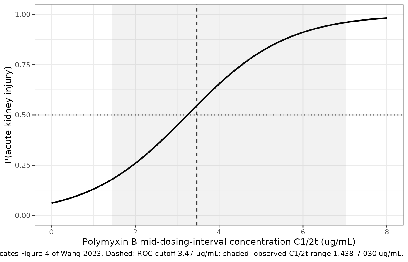
Replicates Figure 4 of Wang 2023.
Figure – multivariable model surface
The paper does not plot Equation 4. The figure shows its predicted probability across the observed AUC range at the Table 1 WBC quartiles. The paper’s cutoff of 0.57 on this probability gave 70% sensitivity and 80% specificity.
eq4_grid <- expand.grid(WBC = c(7.3, 9.6, 13.4), AUC_POLYMYXINB = seq(30, 180, by = 1))
eq4_grid$prob <- prob_aki(mod_aki, eq4_grid)

ggplot(eq4_grid, aes(AUC_POLYMYXINB, prob, colour = factor(WBC))) +
  geom_line(linewidth = 0.9) +
  geom_hline(yintercept = 0.57, linetype = "dashed") +
  scale_y_continuous(limits = c(0, 1)) +
  labs(
    x = "Polymyxin B AUC0-24 by the first-order equation (ug*h/mL)",
    y = "P(acute kidney injury)", colour = "WBC (10^9/L)",
    caption = "Dashed: the paper's Youden-optimal cutoff 0.57 on the predicted probability."
  ) +
  theme_bw() +
  theme(legend.position = "bottom")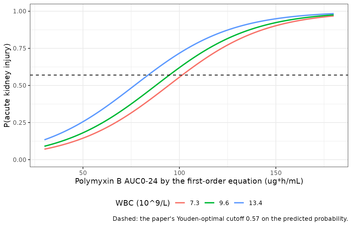
Equation 4 of Wang 2023 at the cohort WBC quartiles.
Generating the exposure inputs from a population PK model
In clinical use, the AUC and the mid-interval concentration come from
therapeutic drug monitoring samples. To show the full chain, this
section simulates steady-state polymyxin B profiles with
Wang_2020_polymyxinB. It then derives the three Wang 2023
exposure metrics from those profiles and passes them to both AKI
models.
Virtual cohort and simulation
The cohort has two maintenance-dose arms of 100 subjects each: 100 mg/day and 150 mg/day, given as 50 mg and 75 mg every 12 h and infused over 1 h. Together these cover 98% of the Wang 2023 patients. Table 1 tabulates the maintenance dose per day; the Methods give it as 2.5-3 mg/kg/day in two divided doses. Creatinine clearance, the only covariate of the PK model, is log-normal and matched to the Table 1 mean +/- SD of 129.6 +/- 62.8 mL/min. Baseline WBC is log-normal and matched to the overall Table 1 median (IQR) of 9.6 (7.3, 13.4) x 10^9/L. Ten doses are given. The 24 h after the 9th dose (96-120 h, the fifth day) are sampled densely, so PKNCA sees a full steady-state day.
rxode2::rxSetSeed(20231)
n_per_arm <- 100
crcl_sdlog <- sqrt(log(1 + (62.8 / 129.6)^2))
wbc_sdlog <- (log(13.4) - log(7.3)) / (2 * stats::qnorm(0.75))

subjects <- tibble::tibble(
  id = seq_len(2 * n_per_arm),
  daily_dose = rep(c(100, 150), each = n_per_arm),
  dose = daily_dose / 2,
  CRCL = exp(stats::rnorm(2 * n_per_arm, log(129.6) - crcl_sdlog^2 / 2, crcl_sdlog)),
  WBC = exp(stats::rnorm(2 * n_per_arm, log(9.6), wbc_sdlog))
) |>
  dplyr::mutate(treatment = paste(daily_dose, "mg/day"))

dose_times <- seq(0, 108, by = 12)
obs_times <- sort(unique(c(seq(96, 120, by = 0.25), 97, 102, 109, 114)))

dose_rows <- subjects |>
  tidyr::crossing(time = dose_times) |>
  dplyr::mutate(amt = dose, rate = dose / 1, evid = 1L, cmt = "central")
obs_rows <- subjects |>
  tidyr::crossing(time = obs_times) |>
  dplyr::mutate(amt = 0, rate = 0, evid = 0L, cmt = "central")
events <- dplyr::bind_rows(dose_rows, obs_rows) |>
  dplyr::arrange(id, time, dplyr::desc(evid)) |>
  dplyr::select(id, time, amt, rate, evid, cmt, CRCL)
sim <- rxode2::rxSolve(mod_pk, events = events, returnType = "data.frame") |>
  as.data.frame() |>
  dplyr::left_join(dplyr::select(subjects, id, treatment, dose, WBC), by = "id")
PKNCA over the steady-state day
conc_df <- sim |>
  dplyr::filter(!is.na(Cc), time >= 96) |>
  dplyr::select(id, treatment, time, Cc) |>
  dplyr::distinct(id, time, .keep_all = TRUE)
dose_df <- dplyr::filter(dose_rows, time >= 96, time < 120) |>
  dplyr::select(id, treatment, time, amt)

conc_obj <- PKNCA::PKNCAconc(conc_df, Cc ~ time | treatment + id)
dose_obj <- PKNCA::PKNCAdose(dose_df, amt ~ time | treatment + id)
intervals <- data.frame(start = 96, end = 120, cmax = TRUE, cmin = TRUE, auclast = TRUE)
nca <- PKNCA::pk.nca(PKNCA::PKNCAdata(conc_obj, dose_obj, intervals = intervals))
nca_wide <- as.data.frame(nca$result) |>
  dplyr::select(id, treatment, PPTESTCD, PPORRES) |>
  tidyr::pivot_wider(names_from = PPTESTCD, values_from = PPORRES)
The Wang 2023 exposure metrics from the simulated samples
The three TDM samples are read off the simulated profile at the Wang 2023 landmarks for a 1-h infusion of the dose at 108 h: the peak at 109 h (end of infusion), C1/2t at 114 h (6 h after the start of the dose) and the trough at 120 h. The AUC is then estimated from the peak and C1/2t by Equations 2-3. The time between the two samples is 5 h; this spacing reproduces the AUC values in the deposited dataset.
# Wang 2023 Equations 2-3 (after Pai 2014): one-compartment first-order
# estimate of the AUC over one dosing interval from two steady-state samples,
# scaled from the 12-h interval to 24 h.
auc_pai_0_24 <- function(cmax, cmid, tinf = 1, tau = 12, dt = 5) {
  ke <- log(cmax / cmid) / dt
  ctrough <- cmax * exp(-ke * (tau - tinf))
  (24 / tau) * (tinf * (cmax + ctrough) / 2 + (cmax - ctrough) / ke)
}

# Known-answer check of the estimator: for a mono-exponential profile after an
# (almost) instantaneous input it is exact, AUC0-tau = C0 * (1 - exp(-k tau)) / k.
k_test <- 0.12
c0_test <- 8
auc_true <- 2 * c0_test * (1 - exp(-k_test * 12)) / k_test
auc_est <- auc_pai_0_24(c0_test, c0_test * exp(-5 * k_test), tinf = 1e-6)
stopifnot(abs(auc_est / auc_true - 1) < 1e-5)

tdm <- sim |>
  dplyr::filter(time %in% c(109, 114, 120)) |>
  dplyr::select(id, treatment, dose, WBC, time, Cc) |>
  tidyr::pivot_wider(names_from = time, values_from = Cc, names_prefix = "c") |>
  dplyr::rename(cmax_tdm = c109, cmid = c114, cmin_tdm = c120) |>
  dplyr::mutate(auc_pai = auc_pai_0_24(cmax_tdm, cmid)) |>
  dplyr::left_join(dplyr::select(nca_wide, id, auclast), by = "id")

pai_ratio <- tdm$auc_pai / tdm$auclast
round(stats::quantile(pai_ratio, c(0.05, 0.5, 0.95)), 3)
#>    5%   50%   95%
#> 0.955 1.001 1.051

stopifnot(
  # The one-compartment two-sample estimate tracks the dense-grid PKNCA AUC of
  # the two-compartment profile closely: by 5 h after the infusion the
  # distribution phase is largely over. The tail quantile is robust to which
  # subjects draw an extreme Q.
  abs(stats::median(pai_ratio) - 1) < 0.10,
  stats::quantile(abs(pai_ratio - 1), 0.9) < 0.25
)
Comparison against the Wang 2023 concentrations
Table 1 reports the observed cohort means. The simulated means are weighted by the Wang 2023 split of daily maintenance doses: 15 patients on 100 mg/day and 39 on 150 mg/day. The one patient on 200 mg/day is not represented.
w <- c(`100 mg/day` = 15, `150 mg/day` = 39)
sim_means <- nca_wide |>
  dplyr::group_by(treatment) |>
  dplyr::summarise(dplyr::across(c(cmax, cmin, auclast), mean)) |>
  dplyr::summarise(dplyr::across(c(cmax, cmin, auclast), ~ sum(.x * w[treatment]) / sum(w)))

reference <- data.frame(cmax = 7.5, cmin = 2.2, auclast = 99.1)

cmp <- nlmixr2lib::ncaComparisonTable(
  simulated = sim_means,
  reference = reference,
  units = c(cmax = "ug/mL", cmin = "ug/mL", auclast = "ug*h/mL, 0-24 h"),
  tolerance_pct = 20
)
knitr::kable(
  cmp,
  digits = 2,
  caption = paste(
    "Dose-weighted mean steady-state NCA from Wang_2020_polymyxinB against the",
    "Wang 2023 Table 1 cohort means. The reference AUC is the three-sample",
    "trapezoidal AUC0-24 (Cmin, C1/2t, Cmax); the simulated AUC uses the full",
    "simulated grid. * differs by more than 20%."
  )
)| NCA parameter | Reference | Simulated | % diff |
|---|---|---|---|
| Cmax (ug/mL) | 7.5 | 7.87 | +4.9% |
| Cmin (ug/mL) | 2.2 | 1.63 | -26.0%* |
| AUClast (ug*h/mL, 0-24 h) | 99.1 | 79.8 | -19.5% |
derived <- tdm |>
  dplyr::group_by(treatment) |>
  dplyr::summarise(cmid = mean(cmid), auc_pai = mean(auc_pai)) |>
  dplyr::summarise(dplyr::across(c(cmid, auc_pai), ~ sum(.x * w[treatment]) / sum(w)))
derived_tbl <- tibble::tibble(
  metric = c("C1/2t (ug/mL)", "AUC0-24 by Equations 2-3 (ug*h/mL)"),
  reference = c(3.6, 91.9),
  simulated = c(derived$cmid, derived$auc_pai)
) |>
  dplyr::mutate(pct_diff = 100 * (simulated / reference - 1))
derived_tbl |>
  dplyr::rename(
    "Exposure metric" = metric, "Wang 2023 Table 1 mean" = reference,
    "Simulated (dose-weighted mean)" = simulated, "% diff" = pct_diff
  ) |>
knitr::kable(digits = 2, caption = "The two exposure inputs of the AKI models: simulated against Wang 2023 Table 1.")| Exposure metric | Wang 2023 Table 1 mean | Simulated (dose-weighted mean) | % diff |
|---|---|---|---|
| C1/2t (ug/mL) | 3.6 | 2.93 | -18.55 |
| AUC0-24 by Equations 2-3 (ug*h/mL) | 91.9 | 80.24 | -12.69 |
The simulated dose-weighted means differ from the Wang 2023 Table 1 means by 5% (Cmax), -26% (Cmin), -19% (C1/2t) and -13% (AUC by Equations 2-3). The PK model was developed in a different cohort, in patients sampled on day 4, so the agreement is a plausibility check of the chain, not a validation of the AKI models.
Predicted AKI risk by maintenance dose
tdm$p_eq4 <- prob_aki(mod_aki, data.frame(WBC = tdm$WBC, AUC_POLYMYXINB = tdm$auc_pai))
tdm$p_eq5 <- prob_aki(mod_cmid, data.frame(CMID_INTERVAL = tdm$cmid))

risk <- tdm |>
  dplyr::group_by(treatment) |>
  dplyr::summarise(
    median_auc = stats::median(auc_pai), median_cmid = stats::median(cmid),
    mean_p_eq4 = mean(p_eq4), mean_p_eq5 = mean(p_eq5)
  ) |>
  dplyr::mutate(observed = c(4 / 15, 25 / 39))

risk |>
  dplyr::rename(
    "Daily maintenance dose" = treatment, "Median AUC0-24 (ug*h/mL)" = median_auc,
    "Median C1/2t (ug/mL)" = median_cmid, "Mean P(AKI), Equation 4" = mean_p_eq4,
    "Mean P(AKI), Equation 5" = mean_p_eq5, "Observed AKI fraction (Table 1)" = observed
  ) |>
knitr::kable(digits = 3, caption = "Simulated exposure and predicted AKI risk by maintenance dose; observed fractions are 4/15 and 25/39 from Wang 2023 Table 1.")| Daily maintenance dose | Median AUC0-24 (ug*h/mL) | Median C1/2t (ug/mL) | Mean P(AKI), Equation 4 | Mean P(AKI), Equation 5 | Observed AKI fraction (Table 1) |
|---|---|---|---|---|---|
| 100 mg/day | 51.495 | 1.849 | 0.314 | 0.331 | 0.267 |
| 150 mg/day | 80.956 | 2.844 | 0.473 | 0.461 | 0.641 |
stopifnot(
  # Both models are monotone in exposure, and 150 mg/day gives 1.5-fold the
  # exposure of 100 mg/day in a linear PK model, so the higher dose must carry the
  # higher mean risk whatever cohort is drawn.
  risk$mean_p_eq4[2] > risk$mean_p_eq4[1],
  risk$mean_p_eq5[2] > risk$mean_p_eq5[1]
)
Assumptions and deviations
-
No residual error and no random effects in the
source. Both regressions have a Bernoulli likelihood. The fixed
additive residual
addSd_prob_aki = 0.001is not a published quantity; it only gives rxode2 an error model to attach to the probability. Use theprob_akicolumn, not a simulated observation, as the model prediction. -
AUC estimator.
AUC_POLYMYXINBis the quantity the regression was fitted to: an AUC0-24 from the peak and C1/2t by the one-compartment first-order equation. Wang 2023 states only that C1/2t was drawn “6 h after administration”. The maintainers found that the AUC values in the deposited dataset are reproduced to within 1.0% when the two samples are taken 5 h apart for every patient, including the seven infused over 2 or 2.5 h. Theauc_pai_0_24()helper above uses that convention. An AUC0-24 from a population PK model can be supplied instead; the simulation above shows the two agree closely for this drug. - Landmark. Both models are static and the probability applies to the whole treatment course. AKI was observed between day 3 and day 17. The paper gives no time course of risk, and the models carry none.
-
Variables screened but not retained. Maintenance
dose, neutrophil percentage, Cmin, Cmax, C1/2t and the AUCs estimated by
the other methods were all significant in univariate analysis. Forward
stepwise selection kept only WBC and the C1/2t-Cmax AUC. These variables
are listed under
covariatesDataExcluded; no coefficients are published for them. -
Female percentage. Table 1 prints “30 (36.7)” for
female patients, which conflicts with 35 male patients out of 55. The
non-AKI and AKI columns (12 and
- sum to 20, so
sex_female_pctis recorded as 20/55 = 36.4%.
- sum to 20, so
-
PK chain. The population PK model is
Wang_2020_polymyxinB, not a model from this paper. Its cohort, creatinine-clearance distribution and day-4 sampling differ from the Wang 2023 cohort. The comparison tables check the chain for plausibility only. The 1-h infusion and the two-arm dose split are simplifications of the Wang 2023 regimens.