Cliramitug (Michalon 2025)
Source:vignettes/articles/Michalon_2025_cliramitug.Rmd
Michalon_2025_cliramitug.RmdModel and source
Cliramitug (development codes NI006 and ALXN2220) is a human IgG1 antibody that binds a cryptic epitope exposed only in transthyretin amyloid (ATTR) fibrils and triggers their removal by phagocytic immune cells. Michalon et al. built a translational PK/PD model to choose the starting dose, dose range and treatment duration of the first-in-human phase Ib study NI006-101. The paper contributes two models:
-
Michalon_2025_cliramitug_rat– the rat two-compartment population PK model (Table 1) whose estimates were allometrically scaled to human. -
Michalon_2025_cliramitug_human_qsp– the human mechanistic PK/PD (QSP) model of cardiac ATTR depletion and left ventricular wall thickness (LVWT).
rat <- rxode2::rxode(readModelDb("Michalon_2025_cliramitug_rat"))
#> ℹ parameter labels from comments will be replaced by 'label()'
hum <- rxode2::rxode(readModelDb("Michalon_2025_cliramitug_human_qsp"))- Citation: Michalon A, Renaud L, Machacek M, Cortijo C, Udata C, Mercuri MF, Buller F, Hock C, Nitsch RM, Kahr PC, Grimm J. Prediction of Cardiac ATTR Depletion by NI006 (ALXN2220) Using Mechanistic PK/PD Modeling. Clin Pharmacol Ther. 2025;117(1):261. doi:10.1002/cpt.3455. Parameter values from Supplementary Table S1 (human PK also Table 1; disease progression also Table S2); ODEs and unit conversions from Supplementary Data S1 ‘Human PK/PD simulations’ Mlxtran code.
- Rat model: Preclinical (rat). Two-compartment population PK model with linear elimination for cliramitug (NI006, ALXN2220), a human IgG1 anti-ATTR amyloid depleter antibody, after intravenous dosing in rats (3 and 30 mg/kg single dose, 300 mg/kg weekly x3). These rat estimates were allometrically scaled to the human PK layer of the companion QSP model Michalon_2025_cliramitug_human_qsp.
- Human model: QSP. Translational mechanistic PK/PD model of cardiac amyloid transthyretin (ATTR) depletion by cliramitug (NI006, ALXN2220) in a typical 70 kg patient with ATTR cardiomyopathy. Two-compartment serum PK allometrically scaled from rat, plus a cardiac-interstitium compartment holding antibody and ATTR; antibody-ATTR binding by the quasi-equilibrium approximation; ATTR formed at a constant rate, cleared spontaneously and by phagocytosis at a rate proportional to the fraction of ATTR bound; excess left ventricular wall thickness (LVWT) proportional to ATTR mass. Population-typical deterministic projection without between-subject variability or residual error.
- Article: https://doi.org/10.1002/cpt.3455 (open access, PMC11652821)
Population
Rat. 36 rats (6 male and 6 female per dose group) received cliramitug IV as a single 3 or 30 mg/kg dose or as three weekly 300 mg/kg doses; serum was sampled from 5 minutes to 28 days after dosing (Methods, Figure 1). The model was fit with SAEM in Monolix.
Human. The human model is a forward projection for a typical 70 kg patient with ATTR cardiomyopathy and a baseline LVWT of 16.6 mm; no patient data were used to fit it. The disease-progression layer was fitted to published LVWT values from untreated ATTR-CM patients aged 30 to 76 years and from the patisiran APOLLO trial. Simulated regimens were 0.3, 1, 3, 10, 30 and 60 mg/kg every 4 weeks as 2-hour infusions, the doses later studied in NI006-101.
str(rat$population)
#> List of 9
#>  $ species       : chr "rat"
#>  $ n_subjects    : int 36
#>  $ n_studies     : int 1
#>  $ weight_range  : chr "Not reported; 0.3 kg used as the rat reference body weight for allometric scaling"
#>  $ sex_female_pct: num 50
#>  $ disease_state : chr "Healthy (cliramitug does not bind native transthyretin; rats carry no ATTR amyloid)"
#>  $ dose_range    : chr "3 or 30 mg/kg IV single dose, or 300 mg/kg IV weekly for 3 doses (12 animals per group, 6 male and 6 female)"
#>  $ regions       : chr "Not reported (GLP toxicology / PK study)"
#>  $ notes         : chr "Serum sampled from 5 min to 28 days post dose with a GLP-qualified assay; in the 300 mg/kg group samples were t"| __truncated__
str(hum$population)
#> List of 8
#>  $ species      : chr "human"
#>  $ n_subjects   : int NA
#>  $ n_studies    : int 0
#>  $ weight_median: chr "70 kg (standard individual; mg/kg doses are multiplied by 70)"
#>  $ disease_state: chr "Transthyretin amyloid cardiomyopathy (ATTR-CM), baseline LVWT 16.6 mm"
#>  $ dose_range   : chr "Simulated 0.3, 1, 3, 10, 30 and 60 mg/kg IV every 4 weeks as a 2-hour infusion for 12 months (Figure 4); the ph"| __truncated__
#>  $ regions      : chr "Not applicable (model-based first-in-human projection)"
#>  $ notes        : chr "Forward projection, not a fit to patient data. Human PK scaled from the rat (Michalon_2025_cliramitug_rat) with"| __truncated__
Source trace
| Equation / parameter | Value | Source location |
|---|---|---|
Rat lcl, lvc, lvp,
lq
|
0.00245 L/day, 0.0144 L, 0.0189 L, 0.0178 L/day | Table 1, rat column |
Rat etalcl, etalvc, etalvp,
etalq
|
21%, 10%, 15%, 18% CV | Table 1, brackets; omega^2 = log(1 + CV^2) |
Rat propSd
|
0 (fixed) | Not reported |
| Rat ODEs | 2-compartment, IV | Data S1 ‘Rat PK’ Mlxtran |
Human lcl, lvc, lvp,
lq
|
0.146 L/day, 3.37 L, 4.42 L, 0.676 L/day | Table S1; Table 1 human column |
bc_heart |
0.102 | Table S1 (Shah 2013) |
v_heart |
0.0488 L | Table S1 (Shah 2012) |
q_heart |
0.372 L/day | Table S1 (Shah 2012) |
kd |
2.5 nM | Table S1 (SPR); Results |
lkelmax |
0.066 1/day | Table S1; Results, Figure 2a |
lkin (kgrowth) |
0.43 mm/year | Table S1, Table S2; Results |
lkout (kel) |
0.053 1/year | Table S1, Table S2; Results |
lvwt_healthy |
8.5 mm | Table S2 |
lvwt0 |
16.6 mm | Methods ‘PK/PD model for predictions’; Results |
attr0 |
1.36 g | Table S1; Methods (1% of 136 g) |
mw_ab, mw_ttr
|
150000, 13750 g/mol | Data S1 ‘Human PK/PD simulations’ |
g_per_mm = attr0 / (lvwt0 - lvwt_healthy) |
0.168 g/mm | Methods LVWT equation; Table S1 ‘k’ |
Micro-constants k1h = bc_heart * q_heart / vc,
kh1 = q_heart / v_heart
|
n/a | Data S1 |
| Quasi-equilibrium free antibody in heart | n/a | Data S1 C_FreeNIh
|
d/dt(central), d/dt(peripheral1),
d/dt(heart_isf), d/dt(total_target)
|
n/a | Data S1 ddt_FreeNIc, ddt_FreeNIp,
ddt_TotNIh, ddt_TotTTRh
|
lvwt = total_target / g_per_mm + lvwt_healthy |
n/a | Data S1 TTRthickness; Methods equation |
Rat PK (Figure 1 and Table 1)
rxode2::rxSetSeed(20251)
bw_rat <- 0.3 # kg; the rat reference weight used for allometric scaling
rat_groups <- tibble::tribble(
  ~group, ~dose_mgkg, ~n_dose, ~horizon,
  "3 mg/kg single", 3, 1, 28,
  "30 mg/kg single", 30, 1, 28,
  "300 mg/kg weekly x3", 300, 3, 42
)
make_rat <- function(g, id_offset) {
  ids <- id_offset + seq_len(12)
  dose <- tidyr::expand_grid(id = ids, time = 7 * (seq_len(g$n_dose) - 1)) |>
    dplyr::mutate(amt = g$dose_mgkg * bw_rat, evid = 1L)
  obs <- tidyr::expand_grid(id = ids, time = c(5 / 1440, seq(0.25, g$horizon, by = 0.25))) |>
    dplyr::mutate(amt = NA_real_, evid = 0L)
  dplyr::bind_rows(dose, obs) |>
    dplyr::mutate(cmt = "central", group = g$group) |>
    dplyr::arrange(id, time, dplyr::desc(evid))
}
ev_rat <- dplyr::bind_rows(lapply(seq_len(nrow(rat_groups)), function(i) {
  make_rat(rat_groups[i, ], id_offset = 12L * (i - 1L))
}))
stopifnot(!anyDuplicated(unique(ev_rat[, c("id", "time", "evid")])))
sim_rat <- rxode2::rxSolve(rat, events = ev_rat, keep = "group", returnType = "data.frame")
ggplot(sim_rat, aes(time, Cc, group = id, colour = group)) +
  geom_line(alpha = 0.6) +
  scale_y_log10() +
  labs(
    x = "Time (day)", y = "Serum cliramitug (ug/mL)", colour = NULL,
    caption = "Replicates Figure 1 of Michalon 2025 (12 simulated rats per group)."
  ) +
  theme_bw()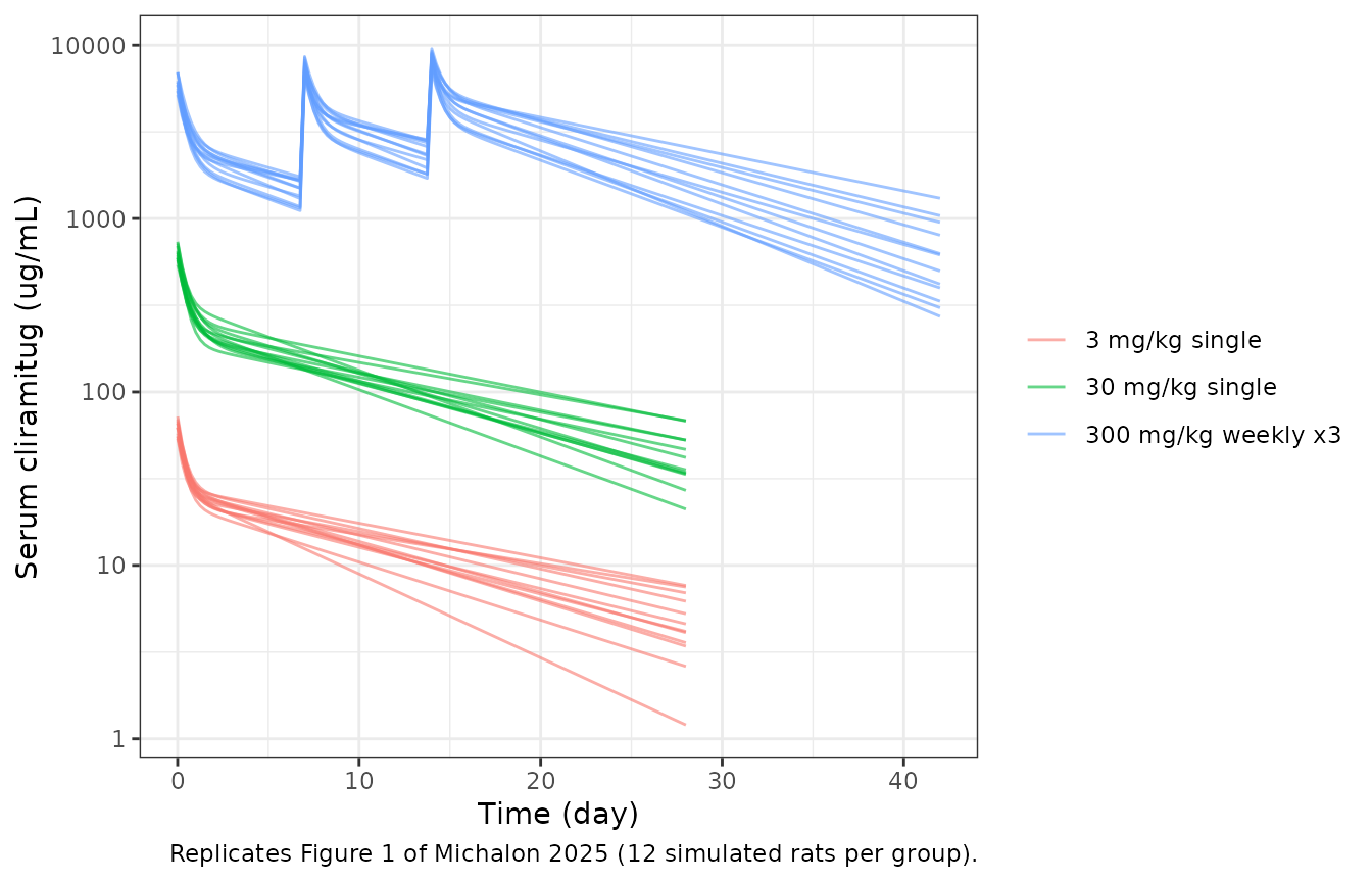
The paper reports no rat NCA; PKNCA summarises the simulated single-dose groups for reference and confirms dose proportionality.
conc_rat <- sim_rat |>
  dplyr::filter(!is.na(Cc), group != "300 mg/kg weekly x3") |>
  dplyr::select(id, time, Cc, group)
conc_rat <- dplyr::bind_rows(
  conc_rat,
  conc_rat |> dplyr::distinct(id, group) |> dplyr::mutate(time = 0, Cc = 0)
) |>
  dplyr::distinct(id, group, time, .keep_all = TRUE) |>
  dplyr::arrange(id, group, time)
dose_rat <- ev_rat |>
  dplyr::filter(evid == 1, group != "300 mg/kg weekly x3") |>
  dplyr::select(id, time, amt, group)
nca_rat <- PKNCA::pk.nca(PKNCA::PKNCAdata(
  PKNCA::PKNCAconc(conc_rat, Cc ~ time | group + id),
  PKNCA::PKNCAdose(dose_rat, amt ~ time | group + id, route = "intravascular"),
  intervals = data.frame(start = 0, end = 28, cmax = TRUE, auclast = TRUE)
))
rat_summary <- as.data.frame(nca_rat) |>
  dplyr::group_by(group, PPTESTCD) |>
  dplyr::summarise(median = median(PPORRES), .groups = "drop") |>
  tidyr::pivot_wider(names_from = PPTESTCD, values_from = median)
rat_summary |>
  dplyr::rename(
    "Group" = group,
    "Cmax (ug/mL)" = cmax,
    "AUC0-28 (ug*day/mL)" = auclast
  ) |>
knitr::kable(digits = 1, caption = "Median simulated rat NCA (single-dose groups).")| Group | AUC0-28 (ug*day/mL) | Cmax (ug/mL) |
|---|---|---|
| 3 mg/kg single | 345.2 | 62.5 |
| 30 mg/kg single | 3318.6 | 625.3 |
# Linear PK: AUC per mg/kg agrees between 3 and 30 mg/kg (between-animal
# variability moves the two group medians by a few percent at most).
auc_per_dose <- rat_summary$auclast / c(3, 30)
stopifnot(abs(auc_per_dose[2] / auc_per_dose[1] - 1) < 0.15)
Allometric scaling to human
The human PK parameters in Table 1 come from the rat values with exponents 1 (V1, V2), 0.75 (Cl) and 2/3 (Q), using 0.3 kg for the rat and 70 kg for human. The check below recomputes them from the packaged rat model and compares them with the packaged human model.
rat_th <- exp(rat$theta[c("lcl", "lvc", "lvp", "lq")])
hum_th <- exp(hum$theta[c("lcl", "lvc", "lvp", "lq")])
scaled <- rat_th * (70 / 0.3)^c(0.75, 1, 1, 2 / 3)
allo <- data.frame(
  parameter = c("Cl (L/day)", "V1 (L)", "V2 (L)", "Q (L/day)"),
  rat = unname(rat_th), scaled = unname(scaled), packaged_human = unname(hum_th)
)
knitr::kable(allo, digits = 4)| parameter | rat | scaled | packaged_human |
|---|---|---|---|
| Cl (L/day) | 0.0025 | 0.1463 | 0.146 |
| V1 (L) | 0.0144 | 3.3600 | 3.370 |
| V2 (L) | 0.0189 | 4.4100 | 4.420 |
| Q (L/day) | 0.0178 | 0.6746 | 0.676 |
Human QSP model
The human simulations are population-typical predictions with no variability. One “month” in the paper’s Figures 4 to 6 is four weeks: doses fall on the integer month ticks of Figure 4a, and 12 doses span the 12-month window.
days_per_month <- 28
dose_levels <- c(0, 0.3, 1, 3, 10, 30, 60)
dose_label <- function(d) ifelse(d == 0, "Placebo", paste(d, "mg/kg"))
make_human <- function(horizon_months = 26) {
  horizon <- horizon_months * days_per_month
  dose <- tidyr::expand_grid(
    dose_mgkg = dose_levels[dose_levels > 0],
    time = seq(0, horizon - days_per_month, by = days_per_month)
  ) |>
    dplyr::mutate(amt = dose_mgkg * 70, dur = 2 / 24, evid = 1L)
  obs <- tidyr::expand_grid(dose_mgkg = dose_levels, time = seq(0, horizon, by = 0.25)) |>
    dplyr::mutate(amt = NA_real_, dur = NA_real_, evid = 0L)
  dplyr::bind_rows(dose, obs) |>
    dplyr::mutate(
      id = match(dose_mgkg, dose_levels),
      treatment = factor(dose_label(dose_mgkg), levels = dose_label(dose_levels)),
      cmt = "central"
    ) |>
    dplyr::arrange(id, time, dplyr::desc(evid))
}
ev_hum <- make_human()
stopifnot(!anyDuplicated(unique(ev_hum[, c("id", "time", "evid")])))

solve_human <- function(params = NULL) {
  rxode2::rxSolve(hum, events = ev_hum, params = params, keep = c("treatment", "dose_mgkg"), returnType = "data.frame") |>
    dplyr::mutate(month = time / days_per_month)
}
sim_base <- solve_human()
Figure 4: serum concentration, ATTR occupancy and LVWT
sim_base |>
  dplyr::filter(month > 0, month <= 12, dose_mgkg > 0) |>
  ggplot(aes(month, Cc, colour = treatment)) +
  geom_line() +
  scale_y_log10() +
  scale_x_continuous(breaks = seq(0, 12, 2)) +
  labs(
    x = "Time (months)", y = "Serum cliramitug (ug/mL)", colour = NULL,
    caption = "Replicates Figure 4a of Michalon 2025."
  ) +
  theme_bw()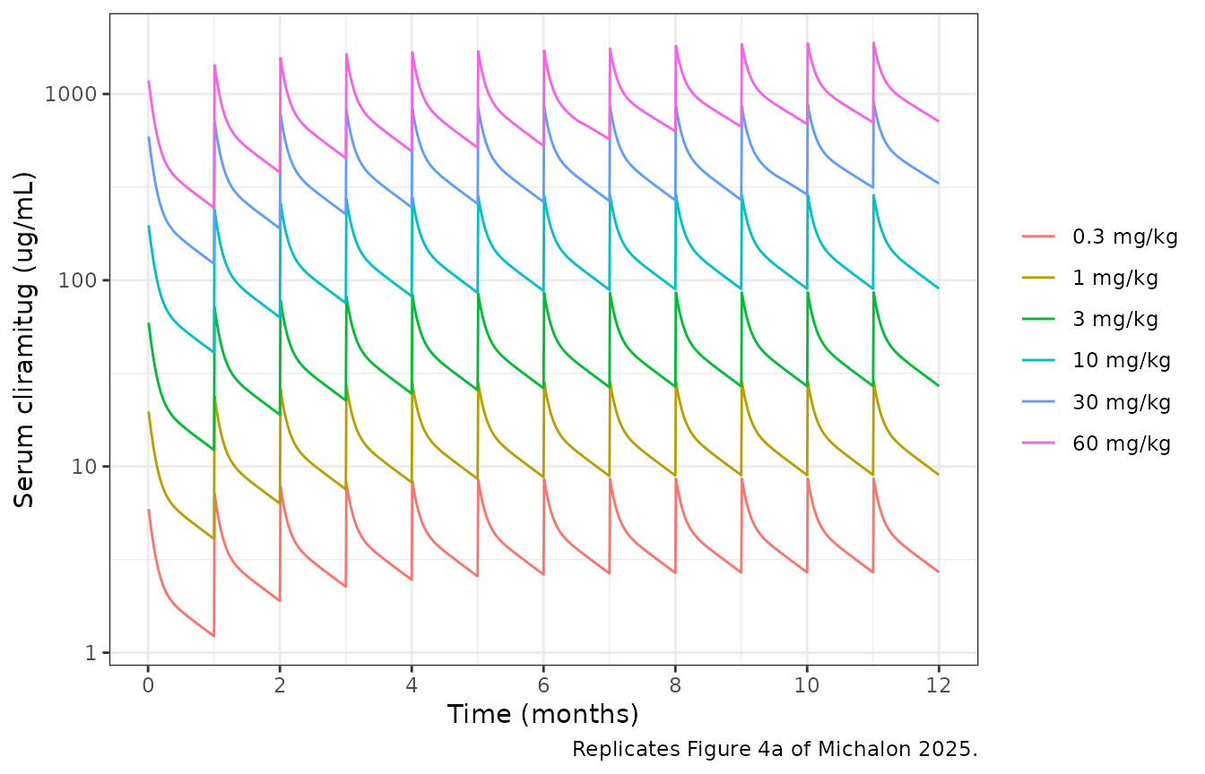
sim_base |>
  dplyr::filter(month <= 12) |>
  ggplot(aes(month, occupancy, colour = treatment)) +
  geom_line() +
  scale_x_continuous(breaks = seq(0, 12, 2)) +
  labs(
    x = "Time (months)", y = "ATTR occupancy (%)", colour = NULL,
    caption = "Replicates Figure 4b of Michalon 2025."
  ) +
  theme_bw()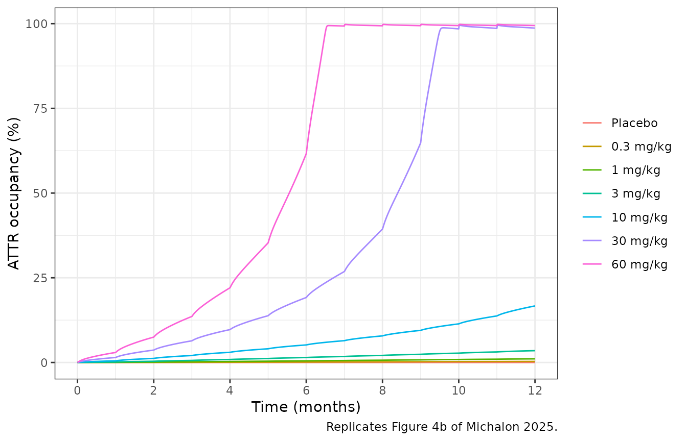
sim_base |>
  dplyr::filter(month <= 12) |>
  ggplot(aes(month, lvwt, colour = treatment)) +
  geom_line() +
  geom_hline(yintercept = 12, linetype = "dashed") +
  scale_x_continuous(breaks = seq(0, 12, 2)) +
  labs(
    x = "Time (months)", y = "Cardiac amyloid surrogate (LVWT, mm)", colour = NULL,
    caption = "Replicates Figure 4c of Michalon 2025; dashed line = 12 mm clinical-effect threshold."
  ) +
  theme_bw()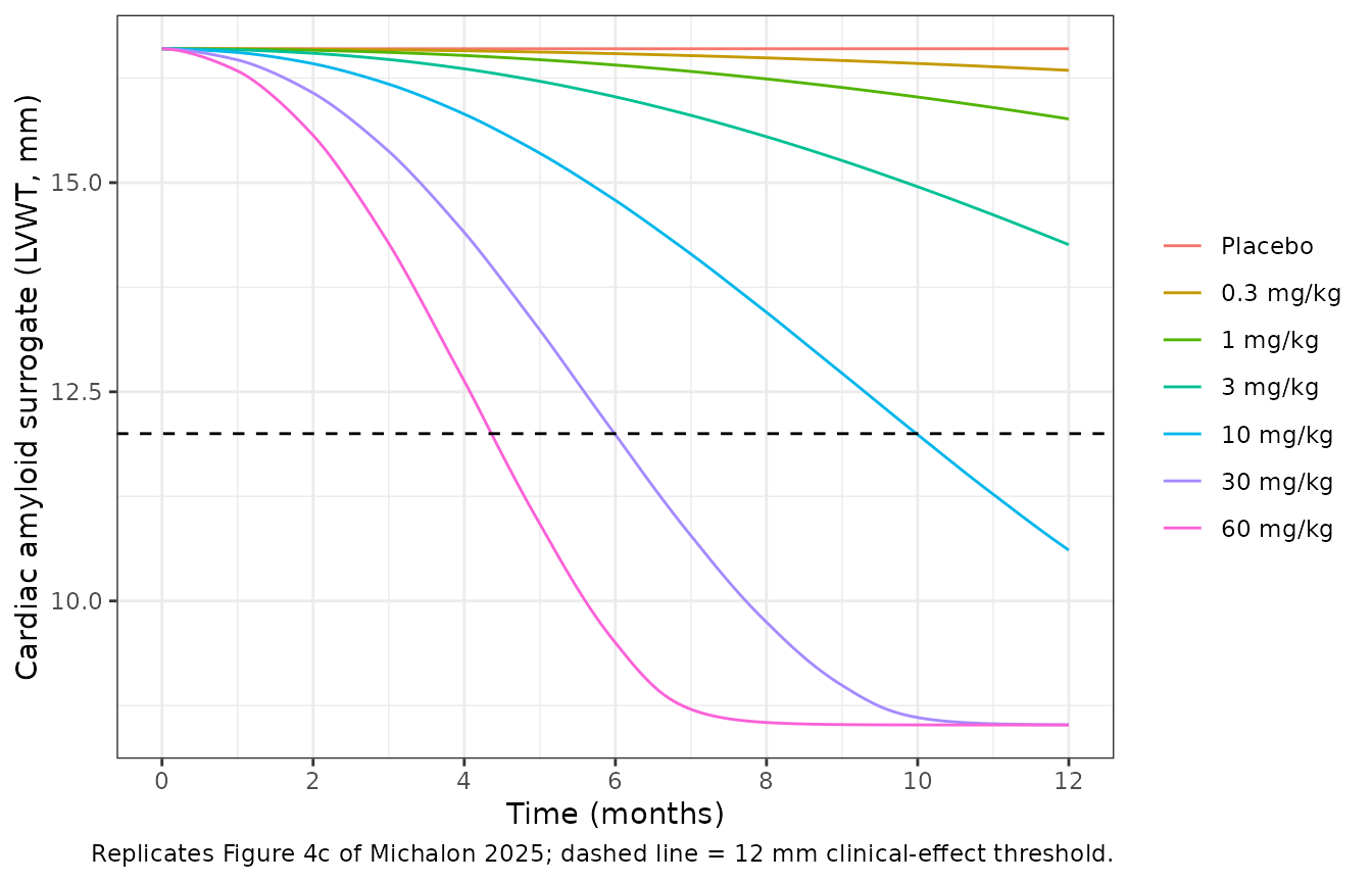
The paper quotes, for the typical patient: a Cmax of 8.4 ug/mL at 0.3 mg/kg with ATTR occupancy below 0.1% after the fourth dose, and 22% occupancy after the fourth monthly 60 mg/kg dose (Results, sensitivity section; Figure 4b).
at_month <- function(sim, m) dplyr::filter(sim, abs(time - m * days_per_month) < 1e-8)
occ4 <- at_month(sim_base, 4)
cmax_4th <- sim_base |>
  dplyr::filter(dose_mgkg == 0.3, time >= 3 * days_per_month, time < 4 * days_per_month) |>
  dplyr::pull(Cc) |>
  max()
cmax_4mo <- sim_base |>
  dplyr::filter(dose_mgkg == 0.3, time <= 4 * days_per_month + 1) |>
  dplyr::pull(Cc) |>
  max()
data.frame(
  quantity = c(
    "Cmax 0.3 mg/kg, 4th dosing interval (ug/mL)",
    "Cmax 0.3 mg/kg, first 4 months incl. the dose at month 4 (ug/mL)",
    "Occupancy 0.3 mg/kg at month 4 (%)",
    "Occupancy 60 mg/kg at month 4 (%)"
  ),
  simulated = c(cmax_4th, cmax_4mo, occ4$occupancy[occ4$dose_mgkg == 0.3], occ4$occupancy[occ4$dose_mgkg == 60]),
  published = c(8.4, 8.4, 0.1, 22)
) |>
knitr::kable(digits = 2)| quantity | simulated | published |
|---|---|---|
| Cmax 0.3 mg/kg, 4th dosing interval (ug/mL) | 8.16 | 8.4 |
| Cmax 0.3 mg/kg, first 4 months incl. the dose at month 4 (ug/mL) | 8.36 | 8.4 |
| Occupancy 0.3 mg/kg at month 4 (%) | 0.09 | 0.1 |
| Occupancy 60 mg/kg at month 4 (%) | 22.04 | 22.0 |
Figure 5: time to clinical effect and sensitivity analyses
Time to clinical effect is the first time LVWT falls below 12 mm. The sensitivity cases raise the baseline cardiac ATTR load 5- and 10-fold (6.8 and 13.6 g) at the same 16.6 mm starting LVWT, or use the 5.6-fold faster xenograft elimination rate (kelmax = 0.37/day).
time_to_effect <- function(sim) {
  sim |>
    dplyr::filter(dose_mgkg > 0) |>
    dplyr::group_by(dose_mgkg) |>
    dplyr::summarise(tte = month[which(lvwt < 12)[1]], .groups = "drop")
}
tte <- dplyr::bind_rows(
  time_to_effect(sim_base) |> dplyr::mutate(scenario = "Base case"),
  time_to_effect(solve_human(c(attr0 = 6.8))) |> dplyr::mutate(scenario = "ATTR load 5x"),
  time_to_effect(solve_human(c(attr0 = 13.6))) |> dplyr::mutate(scenario = "ATTR load 10x"),
  time_to_effect(solve_human(c(lkelmax = log(0.37)))) |> dplyr::mutate(scenario = "kelmax 0.37/day")
)
# Values read from Figure 5 by the maintainers; NA = longer than 26 months.
published_tte <- tibble::tribble(
  ~scenario, ~dose_mgkg, ~tte_pub,
  "Base case", 3, 17.8, "Base case", 10, 10.0, "Base case", 30, 6.0, "Base case", 60, 4.4,
  "ATTR load 5x", 10, 21.8, "ATTR load 5x", 30, 12.7, "ATTR load 5x", 60, 9.2,
  "ATTR load 10x", 30, 17.8, "ATTR load 10x", 60, 12.7,
  "kelmax 0.37/day", 0.3, 23.6, "kelmax 0.37/day", 1, 13.1, "kelmax 0.37/day", 3, 7.8,
  "kelmax 0.37/day", 10, 4.5, "kelmax 0.37/day", 30, 2.7, "kelmax 0.37/day", 60, 2.0
)
tte_cmp <- dplyr::full_join(tte, published_tte, by = c("scenario", "dose_mgkg"))

ggplot(dplyr::filter(tte_cmp, !is.na(tte) | !is.na(tte_pub)), aes(dose_mgkg, tte, colour = scenario)) +
  geom_line() +
  geom_point() +
  geom_point(aes(y = tte_pub), shape = 4, size = 3) +
  scale_x_log10(breaks = c(0.3, 1, 3, 10, 30, 60)) +
  labs(
    x = "Dose (mg/kg every 4 weeks)", y = "Time to clinical effect (months)", colour = NULL,
    caption = "Replicates Figure 5 of Michalon 2025; lines = packaged model, crosses = published."
  ) +
  theme_bw()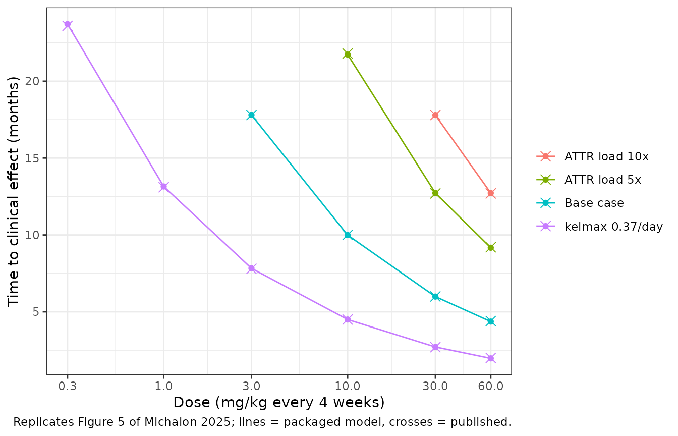
tte_cmp |>
  dplyr::filter(!is.na(tte) | !is.na(tte_pub)) |>
  dplyr::arrange(scenario, dose_mgkg) |>
  dplyr::relocate(scenario) |>
  dplyr::rename(
    "Scenario" = scenario, "Dose (mg/kg)" = dose_mgkg,
    "Simulated (months)" = tte, "Figure 5 (months)" = tte_pub
  ) |>
knitr::kable(digits = 1)| Scenario | Dose (mg/kg) | Simulated (months) | Figure 5 (months) |
|---|---|---|---|
| ATTR load 10x | 30.0 | 17.8 | 17.8 |
| ATTR load 10x | 60.0 | 12.7 | 12.7 |
| ATTR load 5x | 10.0 | 21.7 | 21.8 |
| ATTR load 5x | 30.0 | 12.7 | 12.7 |
| ATTR load 5x | 60.0 | 9.2 | 9.2 |
| Base case | 3.0 | 17.8 | 17.8 |
| Base case | 10.0 | 10.0 | 10.0 |
| Base case | 30.0 | 6.0 | 6.0 |
| Base case | 60.0 | 4.4 | 4.4 |
| kelmax 0.37/day | 0.3 | 23.7 | 23.6 |
| kelmax 0.37/day | 1.0 | 13.2 | 13.1 |
| kelmax 0.37/day | 3.0 | 7.8 | 7.8 |
| kelmax 0.37/day | 10.0 | 4.5 | 4.5 |
| kelmax 0.37/day | 30.0 | 2.7 | 2.7 |
| kelmax 0.37/day | 60.0 | 2.0 | 2.0 |
# Deterministic model, so the only slack needed is the reading precision of
# the figure (about 0.3 month); a missing point on either side must agree.
stopifnot(
  identical(is.na(tte_cmp$tte), is.na(tte_cmp$tte_pub)),
  all(abs(tte_cmp$tte - tte_cmp$tte_pub) < 0.5, na.rm = TRUE)
)
occ4_10x <- at_month(solve_human(c(attr0 = 13.6)), 4)
stopifnot(abs(occ4_10x$occupancy[occ4_10x$dose_mgkg == 60] - 1.8) < 0.2) # Results: 22% -> 1.8%
Figure 6: predicted amyloid change against cumulative exposure
Figure 6 overlays the observed phase Ib imaging changes on the model-predicted relative change in cardiac amyloid (here the change in ATTR mass, equal to the change in excess LVWT) against the predicted cumulative AUC at 4 and 12 months. PKNCA computes the AUCs from the typical-value serum profiles.
conc_hum <- sim_base |>
  dplyr::filter(!is.na(Cc), dose_mgkg > 0, time <= 12 * days_per_month) |>
  dplyr::select(id, time, Cc, treatment)
dose_hum <- ev_hum |>
  dplyr::filter(evid == 1, time <= 12 * days_per_month) |>
  dplyr::select(id, time, amt, treatment)
intervals_hum <- data.frame(
  start = c(0, 0, 3 * days_per_month),
  end = c(4 * days_per_month, 12 * days_per_month, 4 * days_per_month),
  auclast = c(TRUE, TRUE, FALSE),
  cmax = c(FALSE, FALSE, TRUE)
)
nca_hum <- PKNCA::pk.nca(PKNCA::PKNCAdata(
  PKNCA::PKNCAconc(conc_hum, Cc ~ time | treatment + id),
  PKNCA::PKNCAdose(dose_hum, amt ~ time | treatment + id, route = "intravascular"),
  intervals = intervals_hum
))
sim_nca <- as.data.frame(nca_hum) |>
  dplyr::mutate(
    window = dplyr::case_when(
      PPTESTCD == "cmax" ~ "4th dosing interval",
      end == 4 * days_per_month ~ "0-4 months",
      TRUE ~ "0-12 months"
    ),
    # ug*day/mL -> mg*day/mL, the unit of Figure 6
    PPORRES = ifelse(PPTESTCD == "auclast", PPORRES / 1000, PPORRES),
    treatment = as.character(treatment)
  ) |>
  dplyr::select(treatment, window, PPTESTCD, PPORRES)

# AUCs read from the Figure 6 x-axis by the maintainers (log scale, about
# +/-10%); Cmax 8.4 ug/mL from the Results text.
published_nca <- tibble::tribble(
  ~treatment, ~window, ~auclast, ~cmax,
  "0.3 mg/kg", "0-4 months", 0.33, NA,
  "1 mg/kg", "0-4 months", 1.1, NA,
  "3 mg/kg", "0-4 months", 3.4, NA,
  "10 mg/kg", "0-4 months", 11.5, NA,
  "30 mg/kg", "0-4 months", 33, NA,
  "60 mg/kg", "0-4 months", 68, NA,
  "0.3 mg/kg", "0-12 months", 1.3, NA,
  "1 mg/kg", "0-12 months", 4.2, NA,
  "3 mg/kg", "0-12 months", 12.5, NA,
  "10 mg/kg", "0-12 months", 41, NA,
  "30 mg/kg", "0-12 months", 125, NA,
  "60 mg/kg", "0-12 months", 270, NA,
  "0.3 mg/kg", "4th dosing interval", NA, 8.4
)
cmp <- nlmixr2lib::ncaComparisonTable(
  simulated = sim_nca,
  reference = published_nca,
  by = c("treatment", "window"),
  units = c(auclast = "mg*day/mL", cmax = "ug/mL"),
  tolerance_pct = 20
)
knitr::kable(cmp, caption = "Simulated vs. published exposure. * differs from reference by >20%.")| NCA parameter | treatment | window | Reference | Simulated | % diff |
|---|---|---|---|---|---|
| Cmax (ug/mL) | 0.3 mg/kg | 4th dosing interval | 8.4 | 8.16 | -2.8% |
| AUClast (mg*day/mL) | 0.3 mg/kg | 0-4 months | 0.33 | 0.341 | +3.2% |
| AUClast (mg*day/mL) | 0.3 mg/kg | 0-12 months | 1.3 | 1.24 | -4.7% |
| AUClast (mg*day/mL) | 1 mg/kg | 0-4 months | 1.1 | 1.14 | +3.2% |
| AUClast (mg*day/mL) | 1 mg/kg | 0-12 months | 4.2 | 4.13 | -1.7% |
| AUClast (mg*day/mL) | 3 mg/kg | 0-4 months | 3.4 | 3.41 | +0.2% |
| AUClast (mg*day/mL) | 3 mg/kg | 0-12 months | 12.5 | 12.4 | -0.9% |
| AUClast (mg*day/mL) | 10 mg/kg | 0-4 months | 11.5 | 11.4 | -1.3% |
| AUClast (mg*day/mL) | 10 mg/kg | 0-12 months | 41 | 41.3 | +0.7% |
| AUClast (mg*day/mL) | 30 mg/kg | 0-4 months | 33 | 34.1 | +3.2% |
| AUClast (mg*day/mL) | 30 mg/kg | 0-12 months | 125 | 127 | +1.5% |
| AUClast (mg*day/mL) | 60 mg/kg | 0-4 months | 68 | 68.1 | +0.2% |
| AUClast (mg*day/mL) | 60 mg/kg | 0-12 months | 270 | 268 | -0.7% |
change <- dplyr::bind_rows(
  at_month(sim_base, 4) |> dplyr::mutate(window = "0-4 months"),
  at_month(sim_base, 12) |> dplyr::mutate(window = "0-12 months")
) |>
  dplyr::filter(dose_mgkg > 0) |>
  dplyr::mutate(
    pct_change = 100 * (total_target / hum$theta[["attr0"]] - 1),
    treatment = as.character(treatment)
  ) |>
  dplyr::select(treatment, dose_mgkg, window, pct_change) |>
  dplyr::left_join(
    sim_nca |> dplyr::filter(PPTESTCD == "auclast") |> dplyr::select(treatment, window, auc = PPORRES),
    by = c("treatment", "window")
  )
# Model-predicted points read from Figure 6 by the maintainers.
published_change <- tibble::tribble(
  ~dose_mgkg, ~window, ~pct_pub,
  0.3, "0-4 months", 0, 1, "0-4 months", -1, 3, "0-4 months", -3,
  10, "0-4 months", -10, 30, "0-4 months", -27, 60, "0-4 months", -49,
  0.3, "0-12 months", -3, 1, "0-12 months", -10, 3, "0-12 months", -29,
  10, "0-12 months", -74, 30, "0-12 months", -100, 60, "0-12 months", -100
)
change <- dplyr::left_join(change, published_change, by = c("dose_mgkg", "window"))

ggplot(change, aes(auc, pct_change)) +
  geom_line() +
  geom_point(aes(colour = treatment), size = 3) +
  geom_point(aes(y = pct_pub), shape = 4, size = 3) +
  scale_x_log10() +
  facet_wrap(~ factor(window, levels = c("0-4 months", "0-12 months"))) +
  labs(
    x = "Total cliramitug AUC (mg*day/mL)", y = "Relative change from baseline\nin cardiac amyloid (%)",
    colour = NULL, caption = "Replicates the model predictions of Figure 6 of Michalon 2025; crosses = published."
  ) +
  theme_bw()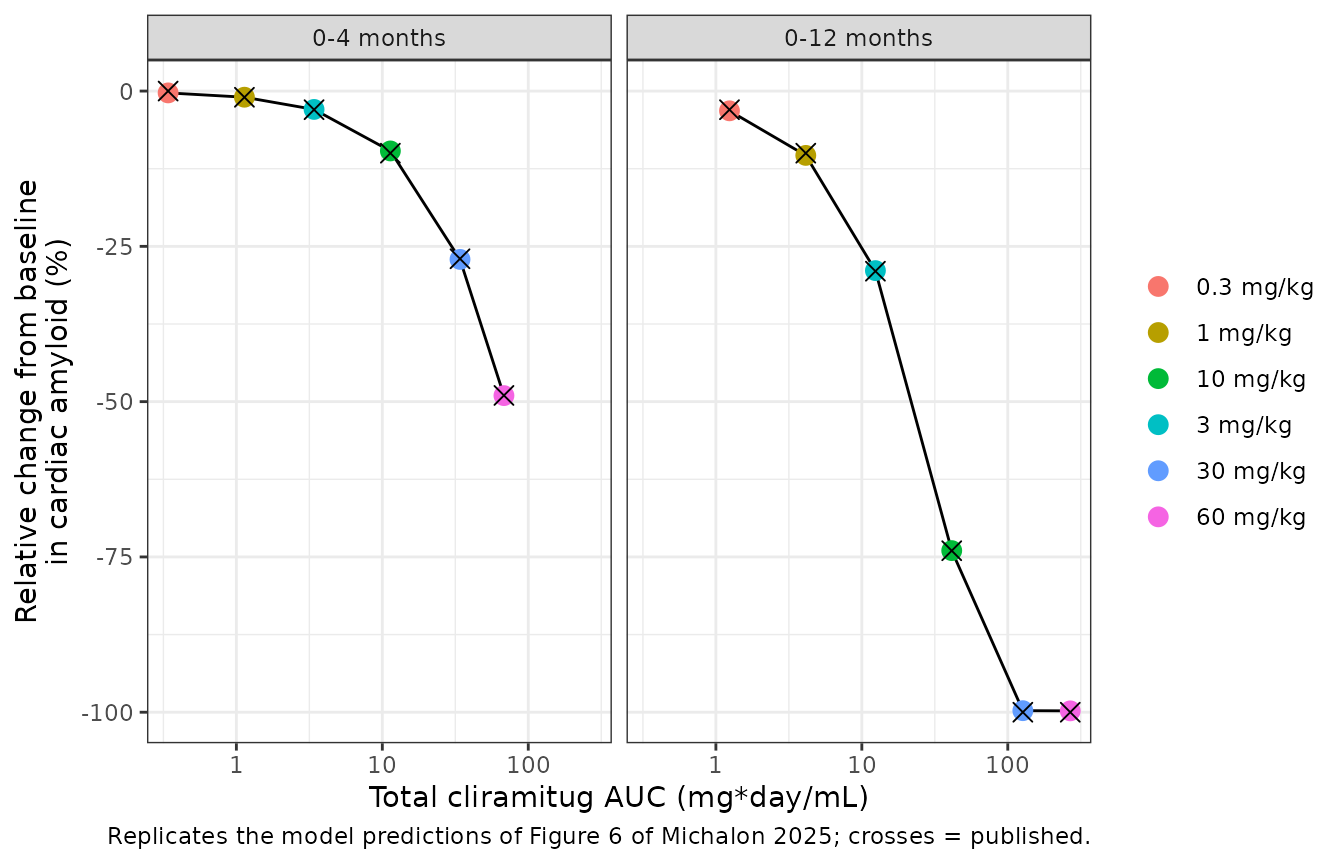
Disease progression (Figure S1)
Without treatment the excess LVWT sits at the steady state of the turnover model, kgrowth / kel = 0.43 / 0.053 = 8.1 mm above the 8.5 mm healthy value, which is the 16.6 mm starting LVWT; the placebo arm in Figure 4c is flat. The spontaneous half-life of excess LVWT is log(2) / 0.053 = 13 years (Results). Patisiran was modelled as an 80% reduction of kgrowth; the right panel of Figure S1 follows a patient from age 60 under that reduction.
stopifnot(all(abs(sim_base$lvwt[sim_base$dose_mgkg == 0] - 16.6) < 0.01))
stopifnot(abs(log(2) / 0.053 - 13) < 0.1)

ev_pat <- data.frame(id = 1L, time = seq(0, 17 * 365.25, by = 30), evid = 0L, cmt = "central")
sim_pat <- rxode2::rxSolve(hum, events = ev_pat, params = c(lkin = log(0.43 * 0.2)), returnType = "data.frame") |>
  dplyr::mutate(age = 60 + time / 365.25)
ggplot(sim_pat, aes(age, lvwt)) +
  geom_line(colour = "red") +
  coord_cartesian(xlim = c(60, 76), ylim = c(0, 20)) +
  labs(
    x = "Age (years)", y = "LVWT (mm)",
    caption = "Replicates the patisiran panel (right) of Figure S1 of Michalon 2025."
  ) +
  theme_bw()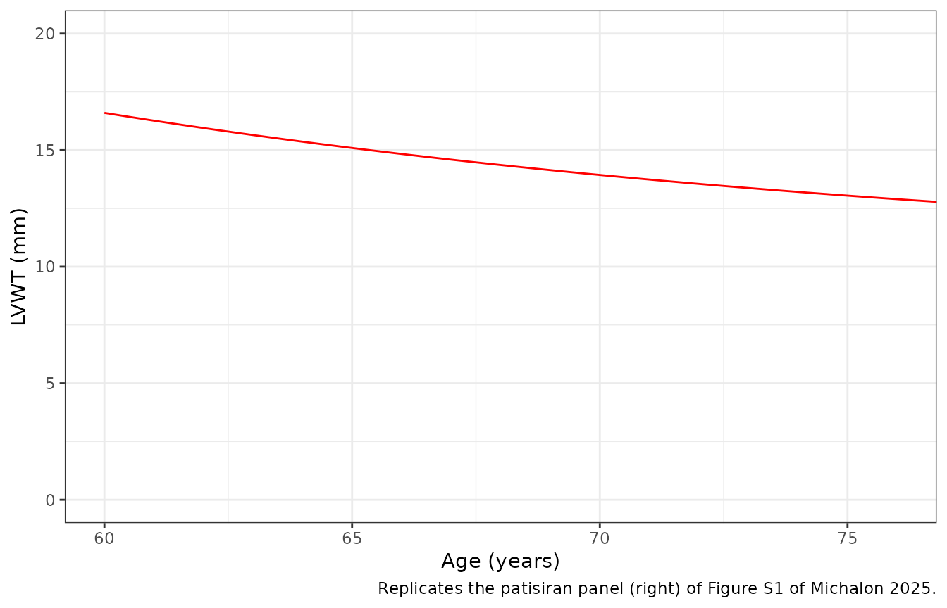
Assumptions and deviations
- Drug name. The paper uses the development codes NI006 and ALXN2220. The files use the INN cliramitug, under which the long-term phase Ib follow-up was published (Nature Medicine 2026); the maintainers verified the assignment on 2026-11-01.
- Disease-progression equation. The Methods print dLVWT/dt = kgrowth - kel * LVWT on total LVWT, whose steady state (0.43 / 0.053 = 8.1 mm) would lie below the healthy 8.5 mm. The deposited Mlxtran code (Data S1) applies the turnover to the excess above 8.5 mm (the ATTR mass), whose steady state is 16.6 mm – the paper’s baseline LVWT and the asymptote of Figure S1. The packaged model follows the code.
-
ATTR state in grams. The code tracks ATTR in nmol
of TTR monomer; the package tracks the same quantity as mass in grams
(
total_target) and converts to nM for binding with the 13750 g/mol monomer weight. The two are identical because every ATTR term is linear in the ATTR amount. Antibody amounts are in mg and are converted to nM with 150000 g/mol, again as in the code. -
LVWT per ATTR mass. Table S1 prints the slope as
(16.6 - 8.5) / (136 * 0.01) = 6 mm/g; the model uses the unrounded
expression (5.96 mm/g, as
attr0 / (lvwt0 - lvwt_healthy)in g/mm). The ATTR load sensitivity cases are reproduced by raisingattr0at a fixed 16.6 mm starting LVWT, which scales the ATTR formation rate with it, asTTRkprod_mass = TTRkprod * g_per_mmdoes in the code. - Year length. kgrowth and kel are reported per year and converted with 365.25 days per year; the paper does not state its conversion.
- Month length. The figures use four-week months (see the human simulation section); reproducing Figures 4 to 6 to within reading precision confirms it.
- Cmax at 0.3 mg/kg. The simulated Cmax in the fourth dosing interval is 8.2 ug/mL; the 8.4 ug/mL quoted by the paper is reached by the dose given at month 4. Both are within 3%.
- Occupancy at 60 mg/kg after the fourth dose. The Results quote both 30% (safe-starting-dose section) and 22% (sensitivity section). Figure 4b and the packaged model give 22% at month 4; the 30% figure is reached during the fifth dosing interval.
-
Fixed versus estimated. In the human model, the
literature and physical constants (heart biodistribution coefficient,
volume and exchange clearance, KD, healthy and baseline LVWT, ATTR mass,
molecular weights) are wrapped in
fixed(). The PK parameters (scaled from the rat fit), kelmax (fitted to the ex vivo assay) and kgrowth and kel (fitted to LVWT data) were estimated within the paper and are left unwrapped, although the human model itself was never fitted. - No variability in the human model. The Mlxtran code accepts log-normal standard deviations for Cl, V1, V2 and Q, but the paper states that all human simulations were population-typical and reports no human values; none are attached. The rat between-animal variability is not carried to human.
- Rat model. The between-animal variability in Table 1 is given as %CV and is converted with omega^2 = log(1 + CV^2). The residual-error model is not reported and is held at zero. The rat strain and body weights are not reported; the vignette doses a 0.3 kg rat, the reference weight used for scaling, and gives the doses as IV boluses because the infusion duration is not reported.
- Sub-models not packaged. The fits that produced kelmax – the ex vivo tissue amyloid depletion assay model and the mouse fibril-xenograft model (Data S1) – are not packaged. Their nuisance parameters (initial amyloid area and area-to-concentration factor; mouse V1, Cl, initial fibril concentration and spontaneous elimination rate) are not reported; only their kelmax estimates (0.066 and 0.37 per day) are, and both are used here.
- Updated phase III model. The Discussion notes that the parameters were later updated with the phase Ib results for phase III design; those values are not published in this paper.
- Errata. No correction notice was found for this article as of 2026-11-01.