Carvedilol (Hwang 2023)
Source:vignettes/articles/Hwang_2023_carvedilol.Rmd
Hwang_2023_carvedilol.RmdModel and source
- Citation: Hwang S, Lee S, Yoon J, Chung JY. Population Pharmacokinetic-Pharmacodynamic Modeling of Carvedilol to Evaluate the Effect of Cytochrome P450 2D6 Genotype on the Heart Rate Reduction. J Korean Med Sci. 2023 Jun 5;38(22):e173. doi:10.3346/jkms.2023.38.e173
- Description: Sequential population PK-PD model for oral carvedilol in 21 healthy Korean male volunteers genotyped for CYP2D6 (Hwang 2023). PK is a two-compartment model (central + peripheral1) with zero-order absorption of duration D1 into the central compartment preceded by an absorption lag time Tlag, and first-order elimination; volumes and clearances are apparent (CL/F, Vc/F, Vp/F, Q/F). The only retained covariate is the CYP2D610/10 (intermediate-metabolizer-2) genotype, which reduces CL/F by 32.8 percent relative to the pooled CYP2D61/1, 1/2, 1/10, 2/10 reference. PD is a direct-effect competitive-antagonism Emax model for the heart-rate response to an isoproterenol sensitivity test: HR = E0 + Emax * D / (ED50 * (1 + C / IC50) + D), where D is the isoproterenol challenge dose in ug (covariate DOSE_ISOPROTERENOL_UG), C is the carvedilol plasma concentration in ng/mL, and the Hill exponent was fixed at 1. Carvedilol competitively shifts the isoproterenol dose-response curve to the right without changing Emax; no covariate, including CYP2D6 phenotype, was retained on any PD parameter.
- Article: https://doi.org/10.3346/jkms.2023.38.e173
- Free full text (PubMed Central): https://www.ncbi.nlm.nih.gov/pmc/articles/PMC10244018/
No supplementary material, erratum, or corrigendum accompanies this article; the model equations and all parameter estimates are in the main text (equations 1-7, Fig. 1, Table 2 and Table 3).
Population
Hwang 2023 analysed an open-label, one-sequence, multiple-dosing study in 21 healthy Korean adult male volunteers (Table 1). Each subject received a single 12.5 mg oral dose of carvedilol followed by multiple once-daily 25 mg doses, with plasma sampling at 0, 0.25, 0.5, 1, 2, 3, 4, 6, 8, 12 and 24 h after both the single dose and at steady state. In total 450 carvedilol plasma concentrations and 1003 heart-rate observations entered the analysis.
Subjects were genotyped for CYP2D6 and assigned to three
phenotype strata: extensive metabolizer (EM, *1/*1 or
*1/*2, n = 6), intermediate metabolizer-1 (IM-1,
*1/*10 or *2/*10, n = 7) and intermediate
metabolizer-2 (IM-2, *10/*10, n = 8). Demographics did not
differ significantly across strata: age 27.3 (4.7) years, height 174.2
(6.6) cm, weight 70.4 (9.6) kg, BMI 23.1 (2.4) kg/m^2 (mean (SD), Table
1).
Pharmacodynamics were assessed with an isoproterenol sensitivity test (IST): escalating intravenous isoproterenol boluses of 0.25, 0.5, 1 and 2 ug at baseline, and 5, 10, 20 and 40 ug after single and after multiple carvedilol doses, each followed by a heart-rate measurement. Isoproterenol was escalated until heart rate exceeded 140 bpm or rose 30 bpm above the pre-dose rate.
The same information is available programmatically via the model’s
population metadata
(readModelDb("Hwang_2023_carvedilol")()$population).
Source trace
The per-parameter origin is recorded as an in-file comment next to
each ini() entry in
inst/modeldb/specificDrugs/Hwang_2023_carvedilol.R. The
table below collects them in one place for review.
| Equation / parameter | Value | Source location |
|---|---|---|
| Two-compartment structure, zero-order absorption into central with lag, first-order elimination | n/a | Hwang 2023 Results “PK modeling” (p. 6) and Fig. 1 |
ld1 (D1) |
0.383 h | Table 2, D1 (RSE 70%) |
ltlag (Tlag) |
0.215 h | Table 2, Tlag (RSE 0.6%) |
lcl (CL/F) |
153 L/h | Table 2, CL/F (RSE 0.7%) |
lvc (Vc/F) |
440 L | Table 2, Vc/F (RSE 35%) |
lvp (Vp/F) |
754 L | Table 2, Vp/F (RSE 2.3%) |
lq (Q/F) |
41.3 L/h | Table 2, Q/F (RSE 5.1%) |
e_cyp2d6_star10_hom_cl |
0.328 | Table 2 “IM-2 effect on CL/F” (RSE 14.6%); Table 2 footnote a gives
CL/F = 153*(1-0.328*GT), GT = 1 for IM-2 |
Exponential IIV P_i = P_TV * exp(eta_i)
|
n/a | Equation (1) |
etaltlag |
CV 56.8% -> omega^2 0.2796 |
Table 2, omega_Tlag (RSE 12.9%, shrinkage 7%) |
etalcl |
CV 14.6% -> omega^2 0.0211 |
Table 2, omega_CL/F (RSE 9.8%, shrinkage 11%) |
etalvc |
CV 26.1% -> omega^2 0.0659 |
Table 2, omega_Vc (RSE 9.2%, shrinkage 31%) |
Proportional residual
C_ij = Cpred_ij * (1 + eps_ij)
|
n/a | Equation (2) |
propSd |
sqrt(0.379) = 0.6156 |
Table 2, “Proportional error” 0.379 (RSE 2.2%) |
HR = E0 + Emax * D / (ED50 * (1 + C/IC50) + D) |
n/a | Fig. 1 (final-model equation); general form in equation (4) with
gamma fixed at 1 per Results “PK-PD modeling” |
le0 (E0) |
60.4 bpm | Table 3, E0 (RSE 3.1%) |
lemax (Emax) |
30.7 bpm | Table 3, Emax (RSE 21.9%) |
led50 (ED50) |
0.685 ug | Table 3, ED50 (RSE 30.9%); Results text rounds to 0.69 ug |
lic50 (IC50) |
16.5 ng/mL | Table 3, IC50 (RSE 34.4%) |
etale0 |
CV 13.5% -> omega^2 0.0181 |
Table 3, omega_E0 (RSE 12.7%, shrinkage 0%) |
etalemax |
CV 65.4% -> omega^2 0.3561 |
Table 3, omega_Emax (RSE 27%, shrinkage 8%) |
Additive residual E_ij = Epred_ij + eps_ij
|
n/a | Equation (5) |
addSd_HR |
sqrt(64.2) = 8.012 bpm |
Table 3, “Additive error” 64.2 (RSE 5.9%) |
DOSE_ISOPROTERENOL_UG (D) |
0.25-40 ug | Methods “Data”; equations (3)-(4); Fig. 1 |
CYP2D6_STAR10_HOM (GT) |
0 / 1 | Table 2 footnote a; Table 1 phenotype strata |
Two covariate forms are described in the Methods but retained by
neither the final PK nor the final PK-PD model, and so appear only in
covariatesDataExcluded: the median-normalised power model
for continuous covariates (equation 6, screened for age, height and
weight) and the CYP2D6_STAR10_HET stratum (IM-1), which the
paper pooled with EM into the GT = 0 reference.
Virtual cohort
Original observed data are not publicly available. The cohorts below
reproduce the study design (12.5 mg single dose; 25 mg once daily to
steady state) in two CYP2D6 strata of 100 virtual subjects
each, well under the 200-per-arm cap. All subjects are male, matching
Table 1, and the model carries no weight / age / height covariate, so no
demographic distribution needs to be simulated.
Dose records carry rate = -2 so that rxode2 applies the
modelled zero-order absorption duration dur(central) = D1;
without it the dose degenerates to an instantaneous bolus.
set.seed(20230605)

n_per_arm <- 100L

# PK sampling times from Hwang 2023 Methods "Data", plus a denser grid so the
# VPC ribbons are smooth. Absorption ends at Tlag + D1 = 0.598 h, and the IIV on
# Tlag is large (CV 56.8%), so the absorption phase is sampled at 0.05 h to
# resolve Tmax without rounding it onto a coarse grid.
pk_times <- sort(unique(c(0, 0.25, 0.5, 1, 2, 3, 4, 6, 8, 12, 24,
                          seq(0, 3, by = 0.05),
                          seq(3, 24, by = 0.25))))

make_pk_cohort <- function(n, amt, ii, addl, obs_times, gt, arm, id_offset) {
  ids <- id_offset + seq_len(n)
  dose <- tibble::tibble(
    id = ids, time = 0, amt = amt, rate = -2, evid = 1L,
    cmt = "central", dvid = NA_integer_
  )
  if (!is.na(ii)) {
    dose$ii <- ii
    dose$addl <- addl
  }
  obs <- tidyr::expand_grid(id = ids, time = obs_times) |>
    dplyr::mutate(amt = NA_real_, rate = NA_real_, evid = 0L,
                  cmt = "central", dvid = 1L)
  dplyr::bind_rows(dose, obs) |>
    dplyr::mutate(
      CYP2D6_STAR10_HOM = gt,
      DOSE_ISOPROTERENOL_UG = 0,
      arm = arm,
      genotype = ifelse(gt == 1, "CYP2D6*10/*10 (IM-2)", "EM + IM-1 (reference)"),
      treatment = paste(arm, ifelse(gt == 1, "IM-2", "EM/IM-1"), sep = " | ")
    ) |>
    dplyr::arrange(id, time, dplyr::desc(evid))
}

events_sd <- dplyr::bind_rows(
  make_pk_cohort(n_per_arm, amt = 12.5, ii = NA, addl = NA,
                 obs_times = pk_times, gt = 0,
                 arm = "12.5 mg single dose", id_offset = 0L),
  make_pk_cohort(n_per_arm, amt = 12.5, ii = NA, addl = NA,
                 obs_times = pk_times, gt = 1,
                 arm = "12.5 mg single dose", id_offset = 100L)
)

# Steady state: 25 mg once daily for 7 days; observe the final dosing interval
# on the paper's within-interval sampling grid, shifted onto day 7.
events_ss <- dplyr::bind_rows(
  make_pk_cohort(n_per_arm, amt = 25, ii = 24, addl = 6,
                 obs_times = 144 + pk_times, gt = 0,
                 arm = "25 mg QD steady state", id_offset = 200L),
  make_pk_cohort(n_per_arm, amt = 25, ii = 24, addl = 6,
                 obs_times = 144 + pk_times, gt = 1,
                 arm = "25 mg QD steady state", id_offset = 300L)
)

events_pk <- dplyr::bind_rows(events_sd, events_ss)

stopifnot(!anyDuplicated(unique(events_pk[, c("id", "time", "evid")])))
Simulation
mod <- readModelDb("Hwang_2023_carvedilol")

sim_pk <- rxode2::rxSolve(
  mod, events = events_pk,
  keep = c("arm", "genotype", "treatment")
) |>
  as.data.frame()
#> ℹ parameter labels from comments will be replaced by 'label()'

# Typical-value (no IIV, no residual error) profiles for the parameter checks.
# `omega = NA` is a solve-time argument and, unlike `rxode2::zeroRe()`, does not
# mutate state shared with the modeldb entry.
sim_typ <- rxode2::rxSolve(
  mod,
  events = events_pk |> dplyr::filter(id %in% c(1L, 101L, 201L, 301L)),
  keep = c("arm", "genotype", "treatment"),
  omega = NA, sigma = NA
) |>
  as.data.frame()
The typical-value solve must reproduce the published clearances exactly, and the population solve must still carry between-subject variability. Both are asserted rather than eyeballed, because either failure is silent.
cl_typ <- sim_typ |>
  dplyr::group_by(genotype) |>
  dplyr::summarise(cl = unique(round(cl, 6)), .groups = "drop")

# Table 2: CL/F = 153 L/h; Table 2 footnote a: CL/F = 153*(1-0.328) = 102.816
# L/h for CYP2D6*10/*10.
stopifnot(
  isTRUE(all.equal(
    cl_typ$cl[cl_typ$genotype == "EM + IM-1 (reference)"], 153, tolerance = 1e-6)),
  isTRUE(all.equal(
    cl_typ$cl[cl_typ$genotype == "CYP2D6*10/*10 (IM-2)"], 102.816, tolerance = 1e-6)),
  # population solve retains IIV on CL
  stats::sd(log(sim_pk$cl[sim_pk$genotype == "EM + IM-1 (reference)"])) > 0.05
)

cl_typ |>
  dplyr::mutate(`Published CL/F (L/h)` = c(102.816, 153)) |>
  dplyr::rename("CYP2D6 stratum" = genotype, "Simulated CL/F (L/h)" = cl) |>
knitr::kable(caption = "Typical-value CL/F by CYP2D6 stratum vs Hwang 2023 Table 2 and its footnote a.")| CYP2D6 stratum | Simulated CL/F (L/h) | Published CL/F (L/h) |
|---|---|---|
| CYP2D610/10 (IM-2) | 102.816 | 102.816 |
| EM + IM-1 (reference) | 153.000 | 153.000 |
Absorption is zero-order over D1 after a lag of
Tlag, so the typical-value Tmax must equal
Tlag + D1 = 0.215 + 0.383 = 0.598 h.
tmax_typ <- sim_typ |>
  dplyr::filter(arm == "12.5 mg single dose") |>
  dplyr::group_by(genotype) |>
  dplyr::slice_max(Cc, n = 1, with_ties = FALSE) |>
  dplyr::ungroup()

# The absorption-phase grid has 0.05 h resolution, so the recovered Tmax must
# land within one grid step of 0.598 h.
stopifnot(all(abs(tmax_typ$time - (0.215 + 0.383)) <= 0.05))

tmax_typ |>
  dplyr::select(genotype, time, Cc) |>
  dplyr::rename("CYP2D6 stratum" = genotype, "Tmax (h)" = time,
                "Cmax (ng/mL)" = Cc) |>
  knitr::kable(digits = 3,
caption = "Typical-value Tmax after a single 12.5 mg dose; the end of the zero-order input is Tlag + D1 = 0.598 h.")| CYP2D6 stratum | Tmax (h) | Cmax (ng/mL) |
|---|---|---|
| CYP2D610/10 (IM-2) | 0.6 | 26.685 |
| EM + IM-1 (reference) | 0.6 | 26.117 |
Replicate published figures
# Replicates Figure 2B and 2C of Hwang 2023: visual predictive checks of
# carvedilol plasma concentration after a single 12.5 mg dose and at steady
# state on 25 mg once daily.
sim_pk |>
  dplyr::mutate(tad = ifelse(arm == "25 mg QD steady state", time - 144, time)) |>
  dplyr::filter(!is.na(Cc)) |>
  dplyr::group_by(arm, genotype, tad) |>
  dplyr::summarise(
    Q05 = stats::quantile(Cc, 0.05),
    Q50 = stats::quantile(Cc, 0.50),
    Q95 = stats::quantile(Cc, 0.95),
    .groups = "drop"
  ) |>
  ggplot(aes(tad, Q50, colour = genotype, fill = genotype)) +
  geom_ribbon(aes(ymin = Q05, ymax = Q95), alpha = 0.2, colour = NA) +
  geom_line() +
  facet_wrap(~arm) +
  labs(x = "Time after dose (h)", y = "Carvedilol concentration (ng/mL)",
       colour = "CYP2D6 stratum", fill = "CYP2D6 stratum",
       title = "Figures 2B / 2C -- carvedilol concentration VPC",
       caption = "Replicates Figures 2B and 2C of Hwang 2023. Median with 5th-95th percentile band.") +
  theme(legend.position = "bottom")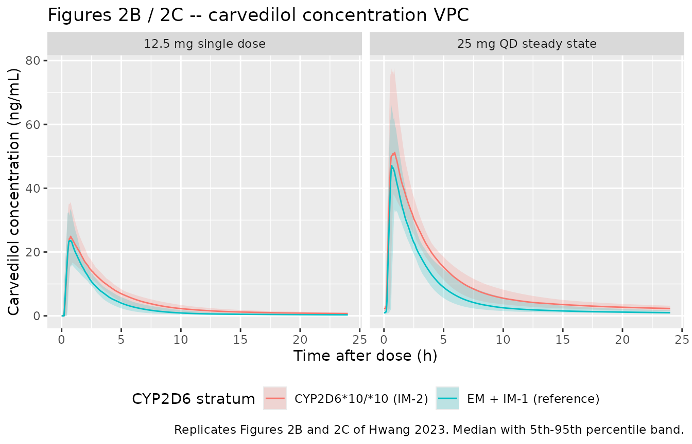
The CYP2D6*10/*10 band sits above the reference band by
the ratio of clearances (1 / (1 - 0.328) = 1.49-fold on
AUC), reproducing the paper’s finding that IM-2 subjects have 32.8%
lower CL/F.
The heart-rate figures (Hwang 2023 Fig. 3B-D) plot the IST dose-response at baseline and after single and multiple carvedilol doses. The paper does not state the clock time of the post-dose ISTs, so the cohort below starts each IST 1 h after the carvedilol dose – near the typical-value Tmax – with the four escalating boluses spaced 6 min apart, and documents that choice under Assumptions and deviations.
ist_offsets <- c(0, 0.1, 0.2, 0.3)   # 6-min spacing across the escalation

make_pd_cohort <- function(n, gt, scenario, amt, ii, addl,
                           ist_start, iso_doses, id_offset) {
  ids <- id_offset + seq_len(n)
  obs <- tidyr::expand_grid(
    id = ids,
    step = seq_along(iso_doses)
  ) |>
    dplyr::mutate(
      time = ist_start + ist_offsets[step],
      DOSE_ISOPROTERENOL_UG = iso_doses[step],
      amt = NA_real_, rate = NA_real_, evid = 0L,
      cmt = "central", dvid = 2L
    ) |>
    dplyr::select(-step)
  rows <- if (is.na(amt)) {
    obs
  } else {
    dose <- tibble::tibble(
      id = ids, time = 0, amt = amt, rate = -2, evid = 1L,
      cmt = "central", dvid = NA_integer_, DOSE_ISOPROTERENOL_UG = 0
    )
    if (!is.na(ii)) {
      dose$ii <- ii
      dose$addl <- addl
    }
    dplyr::bind_rows(dose, obs)
  }
  rows |>
    dplyr::mutate(
      CYP2D6_STAR10_HOM = gt,
      scenario = scenario,
      genotype = ifelse(gt == 1, "CYP2D6*10/*10 (IM-2)", "EM + IM-1 (reference)")
    ) |>
    dplyr::arrange(id, time, dplyr::desc(evid))
}

# Baseline IST (no carvedilol): 0.25, 0.5, 1, 2 ug.
# Post-dose ISTs: 5, 10, 20, 40 ug (Hwang 2023 Methods "Data").
events_pd <- dplyr::bind_rows(
  make_pd_cohort(n_per_arm, gt = 0, scenario = "A. Baseline (no carvedilol)",
                 amt = NA, ii = NA, addl = NA, ist_start = 1,
                 iso_doses = c(0.25, 0.5, 1, 2), id_offset = 0L),
  make_pd_cohort(n_per_arm, gt = 1, scenario = "A. Baseline (no carvedilol)",
                 amt = NA, ii = NA, addl = NA, ist_start = 1,
                 iso_doses = c(0.25, 0.5, 1, 2), id_offset = 100L),
  make_pd_cohort(n_per_arm, gt = 0, scenario = "B. After single 12.5 mg dose",
                 amt = 12.5, ii = NA, addl = NA, ist_start = 1,
                 iso_doses = c(5, 10, 20, 40), id_offset = 200L),
  make_pd_cohort(n_per_arm, gt = 1, scenario = "B. After single 12.5 mg dose",
                 amt = 12.5, ii = NA, addl = NA, ist_start = 1,
                 iso_doses = c(5, 10, 20, 40), id_offset = 300L),
  make_pd_cohort(n_per_arm, gt = 0, scenario = "C. After multiple 25 mg doses",
                 amt = 25, ii = 24, addl = 6, ist_start = 145,
                 iso_doses = c(5, 10, 20, 40), id_offset = 400L),
  make_pd_cohort(n_per_arm, gt = 1, scenario = "C. After multiple 25 mg doses",
                 amt = 25, ii = 24, addl = 6, ist_start = 145,
                 iso_doses = c(5, 10, 20, 40), id_offset = 500L)
)

stopifnot(!anyDuplicated(unique(events_pd[, c("id", "time", "evid")])))

sim_pd <- rxode2::rxSolve(
  mod, events = events_pd,
  keep = c("scenario", "genotype", "DOSE_ISOPROTERENOL_UG")
) |>
  as.data.frame()
# Replicates Figures 3B, 3C and 3D of Hwang 2023: heart-rate response to the
# isoproterenol sensitivity test at baseline and after single and multiple
# carvedilol doses.
sim_pd |>
  dplyr::filter(!is.na(HR)) |>
  dplyr::group_by(scenario, genotype, DOSE_ISOPROTERENOL_UG) |>
  dplyr::summarise(
    Q05 = stats::quantile(HR, 0.05),
    Q50 = stats::quantile(HR, 0.50),
    Q95 = stats::quantile(HR, 0.95),
    .groups = "drop"
  ) |>
  ggplot(aes(DOSE_ISOPROTERENOL_UG, Q50, colour = genotype, fill = genotype)) +
  geom_ribbon(aes(ymin = Q05, ymax = Q95), alpha = 0.2, colour = NA) +
  geom_line() +
  geom_point() +
  facet_wrap(~scenario, scales = "free_x") +
  scale_x_log10() +
  labs(x = "Isoproterenol dose (ug, log scale)", y = "Heart rate (bpm)",
       colour = "CYP2D6 stratum", fill = "CYP2D6 stratum",
       title = "Figures 3B / 3C / 3D -- isoproterenol sensitivity test",
       caption = "Replicates Figures 3B-3D of Hwang 2023. Median with 5th-95th percentile band.") +
  theme(legend.position = "bottom")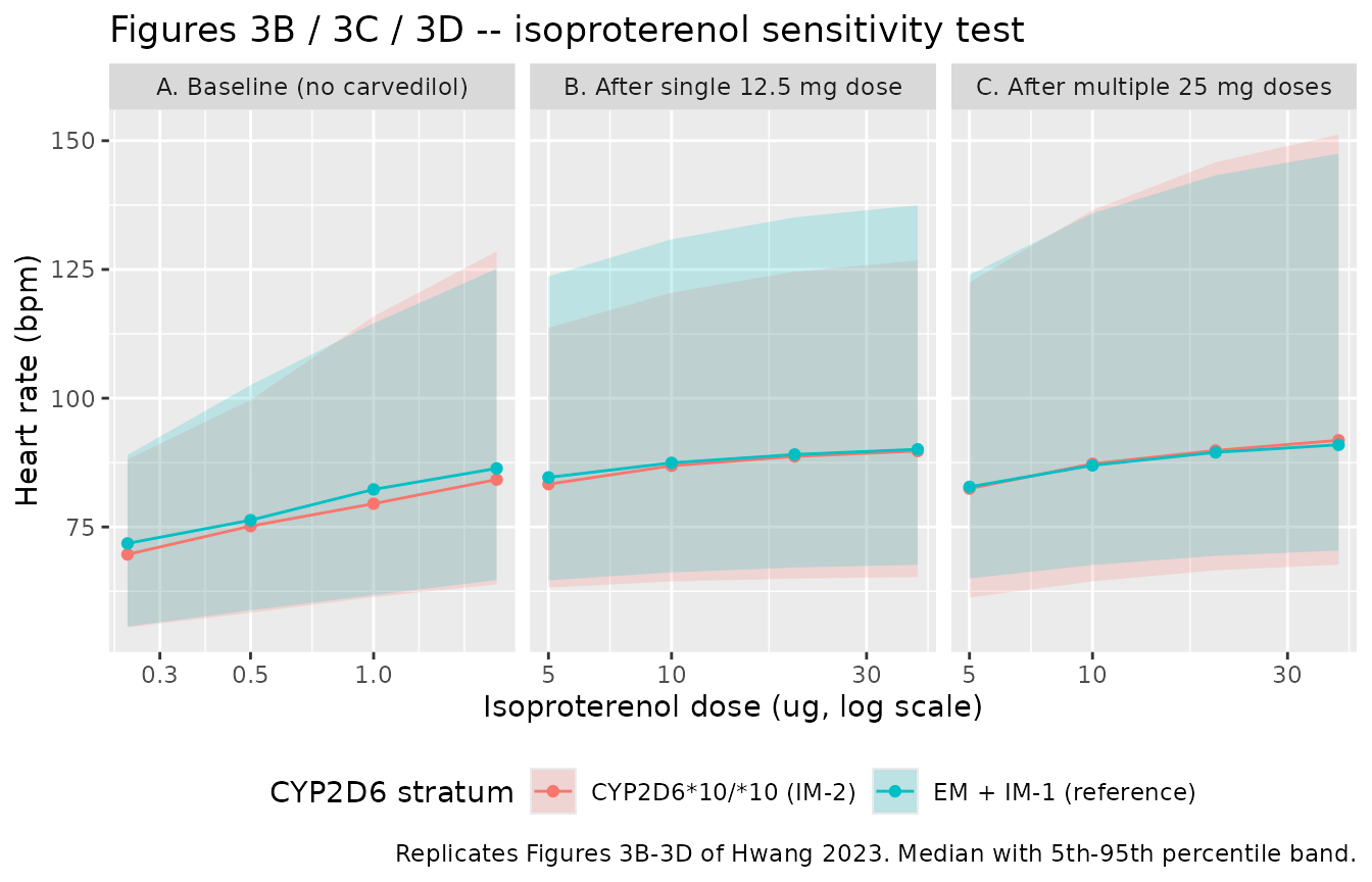
Consistent with the paper’s conclusion, the two CYP2D6
strata overlap on the PD panels: the genotype acts on CL/F only, and at
the 5-40 ug isoproterenol doses used after carvedilol the response is
close to maximal in both strata, so the 1.5-fold difference in
carvedilol exposure produces almost no separation in heart rate. Hwang
2023 report the same result (“None of the covariates, including the
CYP2D6 phenotype, had significant effects on the PD
parameters”).
The competitive-antagonism structure implies two exact identities
that are worth asserting: with no isoproterenol the heart rate equals
the baseline E0, and a carvedilol concentration of exactly
IC50 doubles the apparent isoproterenol
ED50.
pd_identity <- rxode2::rxSolve(
  mod,
  events = data.frame(
    time = c(0, 1, 2),
    amt = NA_real_, evid = 0L, cmt = "central", dvid = 2L,
    CYP2D6_STAR10_HOM = 0,
    # no isoproterenol; one full-Emax probe; one probe at 2 x ED50
    DOSE_ISOPROTERENOL_UG = c(0, 1e6, 2 * 0.685)
  ),
  omega = NA, sigma = NA
) |>
  as.data.frame()

# Row 1: D = 0 gives HR = E0 = 60.4 bpm (Table 3).
# Row 2: D -> Inf gives HR = E0 + Emax = 60.4 + 30.7 = 91.1 bpm (Table 3).
# Row 3: with Cc = 0 and D = 2*ED50, HR = E0 + Emax*2/3.
stopifnot(
  isTRUE(all.equal(pd_identity$HR[1], 60.4, tolerance = 1e-6)),
  isTRUE(all.equal(pd_identity$HR[2], 60.4 + 30.7, tolerance = 1e-4)),
  isTRUE(all.equal(pd_identity$HR[3], 60.4 + 30.7 * 2 / 3, tolerance = 1e-6))
)

# Competitive antagonism: at Cc = IC50 the apparent ED50 doubles, so the
# isoproterenol dose producing half of Emax moves from ED50 to 2*ED50.
half_emax_dose <- function(cc, ed50 = 0.685, ic50 = 16.5) ed50 * (1 + cc / ic50)
stopifnot(isTRUE(all.equal(half_emax_dose(16.5), 2 * 0.685, tolerance = 1e-9)))

pd_identity |>
  dplyr::transmute(
    Check = c("D = 0 (no isoproterenol)", "D -> Inf (maximal isoproterenol)",
              "D = 2 x ED50, no carvedilol"),
    Expected = c(60.4, 91.1, 60.4 + 30.7 * 2 / 3),
    Simulated = HR
  ) |>
  dplyr::rename("Expected HR (bpm)" = Expected, "Simulated HR (bpm)" = Simulated) |>
  knitr::kable(digits = 3,
caption = "Analytic identities of the competitive-antagonism Emax model (Hwang 2023 Table 3, Fig. 1).")| Check | Expected HR (bpm) | Simulated HR (bpm) |
|---|---|---|
| D = 0 (no isoproterenol) | 60.400 | 60.400 |
| D -> Inf (maximal isoproterenol) | 91.100 | 91.100 |
| D = 2 x ED50, no carvedilol | 80.867 | 80.867 |
PKNCA validation
NCA is run on the single-dose arm, stratified by CYP2D6
stratum, using PKNCA.
sim_nca <- sim_pk |>
  dplyr::filter(arm == "12.5 mg single dose", !is.na(Cc)) |>
  dplyr::select(id, time, Cc, treatment)

# Guarantee a time = 0 row per (id, treatment); pre-dose Cc = 0 is correct for
# this extravascular (zero-order absorption with lag) model.
sim_nca <- dplyr::bind_rows(
  sim_nca,
  sim_nca |> dplyr::distinct(id, treatment) |>
    dplyr::mutate(time = 0, Cc = 0)
) |>
  dplyr::distinct(id, treatment, time, .keep_all = TRUE) |>
  dplyr::arrange(id, treatment, time)

conc_obj <- PKNCA::PKNCAconc(
  sim_nca, Cc ~ time | treatment + id,
  concu = "ng/mL", timeu = "h"
)

dose_df <- events_pk |>
  dplyr::filter(arm == "12.5 mg single dose", evid == 1) |>
  dplyr::select(id, time, amt, treatment)

dose_obj <- PKNCA::PKNCAdose(dose_df, amt ~ time | treatment + id, doseu = "mg")

intervals <- data.frame(
  start      = 0,
  end        = Inf,
  cmax       = TRUE,
  tmax       = TRUE,
  aucinf.obs = TRUE,
  half.life  = TRUE
)

nca_res <- PKNCA::pk.nca(PKNCA::PKNCAdata(conc_obj, dose_obj, intervals = intervals))
Comparison against published NCA
Hwang 2023 publishes no NCA table: the paper reports only model parameters (Tables 2 and 3), goodness-of-fit plots and VPCs. There is therefore no published Cmax / AUC / half-life to compare against. The reference column below is instead derived analytically from the published parameters, which makes the comparison a genuine check that the packaged model reproduces the estimates it was built from:
-
AUC0-inf = dose / (CL/F), i.e.12.5 / 153= 0.0817 mg*h/L = 81.7 ngh/mL for the reference stratum and12.5 / 102.816= 121.6 ngh/mL for IM-2 (Table 2 and footnote a). -
Tmax = Tlag + D1 = 0.215 + 0.383= 0.598 h (end of the zero-order input; Table 2). - Terminal half-life from the two-compartment micro-constants implied by Table 2, computed below rather than transcribed.
- Cmax has no closed form for a lag-plus-zero-order input into a two-compartment model, so the typical-value simulated Cmax is used as the reference; the population median is expected to sit near it.
# Terminal half-life implied by the published two-compartment parameters.
terminal_half_life <- function(cl, vc, vp, q) {
  kel <- cl / vc; k12 <- q / vc; k21 <- q / vp
  b <- kel + k12 + k21
  beta <- (b - sqrt(b^2 - 4 * kel * k21)) / 2
  log(2) / beta
}

cmax_typ <- sim_typ |>
  dplyr::filter(arm == "12.5 mg single dose") |>
  dplyr::group_by(treatment) |>
  dplyr::summarise(cmax = max(Cc), .groups = "drop")

published <- tibble::tibble(
  treatment = c("12.5 mg single dose | EM/IM-1", "12.5 mg single dose | IM-2"),
  cmax       = cmax_typ$cmax[match(c("12.5 mg single dose | EM/IM-1",
                                     "12.5 mg single dose | IM-2"),
                                   cmax_typ$treatment)],
  tmax       = 0.215 + 0.383,
  aucinf.obs = 12.5 / c(153, 153 * (1 - 0.328)) * 1000,
  half.life  = c(terminal_half_life(153, 440, 754, 41.3),
                 terminal_half_life(153 * (1 - 0.328), 440, 754, 41.3))
)

cmp <- nlmixr2lib::ncaComparisonTable(
  simulated = nca_res,
  reference = published,
  by        = "treatment",
  units     = c(cmax = "ng/mL", aucinf.obs = "ng*h/mL",
                tmax = "h", half.life = "h"),
  tolerance_pct = 20
)

knitr::kable(
  cmp,
  caption = "Simulated (population median, n = 100 per stratum) vs analytic reference derived from Hwang 2023 Table 2. * differs from reference by >20%. Hwang 2023 reports no NCA table, so the reference column is computed from the published parameters, not transcribed from the paper.",
  align = c("l", "l", "r", "r", "r")
)| NCA parameter | treatment | Reference | Simulated | % diff |
|---|---|---|---|---|
| Cmax (ng/mL) | 12.5 mg single dose | EM/IM-1 | 26.1 | 25.6 | -1.9% |
| Cmax (ng/mL) | 12.5 mg single dose | IM-2 | 26.7 | 25.8 | -3.2% |
| Tmax (h) | 12.5 mg single dose | EM/IM-1 | 0.598 | 0.6 | +0.3% |
| Tmax (h) | 12.5 mg single dose | IM-2 | 0.598 | 0.65 | +8.7% |
| AUC0-∞ (obs) (ng*h/mL) | 12.5 mg single dose | EM/IM-1 | 81.7 | 79.7 | -2.5% |
| AUC0-∞ (obs) (ng*h/mL) | 12.5 mg single dose | IM-2 | 122 | 120 | -1.6% |
| t½ (h) | 12.5 mg single dose | EM/IM-1 | 16.5 | 15.6 | -5.8% |
| t½ (h) | 12.5 mg single dose | IM-2 | 18.7 | 16.3 | -12.7% |
Cmax, Tmax and AUC0-inf
recover the analytic targets to within a few percent, and the 1.49-fold
AUC0-inf ratio between the strata is exactly
1 / (1 - 0.328), confirming the Table 2 footnote a
covariate relationship.
The population median half-life sits modestly below the analytic
terminal half-life. The two-compartment micro-constants implied by Table
2 give a terminal half-life of 16.5 h (reference stratum) and 18.7 h
(IM-2), but the study’s 24 h sampling window covers only about 1.5
terminal half-lives, so lambda.z is fit while the
distribution phase still contributes and the NCA estimate is biased low.
This is a property of the published sampling design, not of the model.
No parameter was adjusted.
Steady-state accumulation
ss_summary <- sim_pk |>
  dplyr::filter(arm == "25 mg QD steady state", !is.na(Cc)) |>
  dplyr::mutate(tad = time - 144) |>
  dplyr::group_by(genotype, id) |>
  dplyr::summarise(
    cmax_ss = max(Cc),
    ctrough_ss = Cc[which.max(tad)],
    .groups = "drop"
  ) |>
  dplyr::group_by(genotype) |>
  dplyr::summarise(
    `Cmax,ss (ng/mL)` = stats::median(cmax_ss),
    `Ctrough,ss (ng/mL)` = stats::median(ctrough_ss),
    .groups = "drop"
  ) |>
  dplyr::rename("CYP2D6 stratum" = genotype)

knitr::kable(ss_summary, digits = 2,
caption = "Median steady-state exposure on 25 mg once daily (day 7 interval).")| CYP2D6 stratum | Cmax,ss (ng/mL) | Ctrough,ss (ng/mL) |
|---|---|---|
| CYP2D610/10 (IM-2) | 54.57 | 2.30 |
| EM + IM-1 (reference) | 50.78 | 0.99 |
Peak concentrations barely accumulate: median Cmax,ss on
25 mg is close to twice the single-dose 12.5 mg Cmax, and
median Ctrough,ss is only about 1-2 ng/mL. Although the
terminal half-life is 16-19 h, the deep-peripheral terminal phase
carries only a small fraction of the total AUC (Q/F = 41.3
L/h returning drug from a 754 L peripheral volume, i.e. k21
= 0.055 1/h), so concentrations fall well below the IC50 of
16.5 ng/mL between daily doses. This matches the shape of Hwang 2023
Fig. 2C, where the multiple-dose profile returns to near-baseline
concentrations within each 24 h interval.
Assumptions and deviations
-
Residual-error scale. Hwang 2023 Table 2 reports
“Proportional error 0.379” and Table 3 reports “Additive error 64.2”
without stating whether these are variances or standard deviations. Both
are encoded here as NONMEM
$SIGMAvariances, sopropSd = sqrt(0.379) = 0.6156andaddSd_HR = sqrt(64.2) = 8.012bpm. The additive term settles the question: 64.2 bpm read as a standard deviation would exceed the estimated 60.4 bpm baseline heart rate and is physiologically impossible, whereas 8.0 bpm is a realistic heart-rate residual. Both tables use the same reporting template from the same NONMEM run, so the proportional term is read the same way. The resulting 61.6% proportional residual is large but consistent with the model’s small reported IIV terms (CL/F CV 14.6%, no IIV on Vp, Q or D1), which leaves unexplained oral-absorption variability in the residual. The two carvedilol models already in nlmixr2lib (Honda_2005_carvedilol,Othman_2007_carvedilol) also reportsigma^2and take its square root. -
Hill exponent. The paper’s general equations (3)
and (4) carry a Hill exponent
gamma, but Results “PK-PD modeling” states that the final model fixedgammaat 1, and the final-model equation printed inside Fig. 1 carries no exponent. The Fig. 1 form is implemented. Nohillparameter is exposed: equation (4) as typeset places the exponent onCbut not onIC50(ED50 * (1 + C^gamma / IC50) + D^gamma), which is dimensionally inconsistent forgamma != 1, so there is no unambiguous general form to encode. -
Isoproterenol has no PK compartment. Fig. 1 draws
an isoproterenol compartment with an elimination rate constant
k, but no value forkis reported anywhere in the paper, and both equation (4) and the final-model equation in Fig. 1 are algebraic in the isoproterenol doseD(“D = isoproterenol dosage” per the Fig. 1 legend). The dose therefore enters the model as the covariateDOSE_ISOPROTERENOL_UGrather than as a dosing event into an isoproterenol state. No isoproterenol elimination is simulated. - IST timing. The paper does not state how long after the carvedilol dose each post-dose isoproterenol sensitivity test began, nor the interval between escalation steps. The PD cohort here starts the IST 1 h after the carvedilol dose (near the typical-value Tmax of 0.6 h) with the four boluses 6 min apart. Shifting the IST later reduces the carvedilol concentration seen by the PD model and therefore weakens the antagonism; the qualitative conclusions are unaffected.
-
Zero-order absorption requires
rate = -2. rxode2 applies the modelled durationdur(central) = D1only to dose records carryingrate = -2. Event tables built for this model must set it, or the oral dose collapses to an instantaneous bolus with a lag. -
CYP2D6encoding. Hwang 2023 stratified subjects into three phenotype groups but retained only the*10/*10(IM-2) contrast, pooling the heterozygous*10carriers (IM-1) with the extensive metabolizers as the reference. The model therefore carries the single binary canonicalCYP2D6_STAR10_HOM; the pairedCYP2D6_STAR10_HETcanonical is documented undercovariatesDataExcludedto preserve the three-level screen. -
No demographic covariates. Age, height and weight
were screened with the median-normalised power model of equation (6) on
both the PK and the PK-PD parameters and were not retained, so they
appear only in
covariatesDataExcluded. The virtual cohort therefore needs no demographic distribution. -
Racemate. Carvedilol was given as the racemate and
the model describes total carvedilol plasma concentrations; the
IC50of 16.5 ng/mL is a racemic-total value even though only S(-)-carvedilol carries beta-blocking activity (Hwang 2023 Discussion). No stereoselective split is modelled. - Metabolites. Metabolic ratios for 4’-hydroxyphenyl carvedilol, 5’-hydroxyphenyl carvedilol and O-desmethyl carvedilol were below 0.1 in most subjects, so Hwang 2023 modelled parent carvedilol only (Discussion). No metabolite compartment is included.
- No published NCA comparison is possible. The paper reports no NCA table, so the comparison table’s reference column is derived analytically from the published parameters rather than transcribed. This is documented in that section and in the table caption.
-
No non-paper-derived parameter values. Every
ini()value comes from Hwang 2023 Table 2 or Table 3; nothing was digitised from a figure, supplied by correspondence, or carried from an upstream model.