Methylprednisolone IL-6 and IL-10 in neonatal cardiopulmonary bypass (Hornik 2019)
Source:vignettes/articles/Hornik_2019_methylprednisolone.Rmd
Hornik_2019_methylprednisolone.RmdModel and source
Hornik 2019 developed one population PK model of methylprednisolone and two separate sequential PK/PD models, one for interleukin-6 (IL-6) and one for interleukin-10 (IL-10). Each PK/PD model is packaged as its own file carrying the shared PK model:
-
Hornik_2019_methylprednisolone_il6: Two-compartment population PK model of methylprednisolone with first-order formation from its sodium succinate prodrug, linked to an indirect-response model of interleukin-6 (IL-6) in which methylprednisolone inhibits and cardiopulmonary bypass (CPB) stimulates IL-6 production with partial drug-CPB interaction, in neonates undergoing cardiac surgery on CPB (Hornik 2019) -
Hornik_2019_methylprednisolone_il10: Two-compartment population PK model of methylprednisolone with first-order formation from its sodium succinate prodrug, linked to an indirect-response model of interleukin-10 (IL-10) in which methylprednisolone and cardiopulmonary bypass (CPB) both stimulate IL-10 production with complete (multiplicative) drug-CPB interaction, in neonates undergoing cardiac surgery on CPB (Hornik 2019) - Citation: Hornik CP, Gonzalez D, Dumond J, Wu H, Graham EM, Hill KD, Cohen-Wolkowiez M. Population Pharmacokinetic/Pharmacodynamic Modeling of Methylprednisolone in Neonates Undergoing Cardiopulmonary Bypass. CPT Pharmacometrics Syst Pharmacol. 2019;8(12):913-922. doi:10.1002/psp4.12470
- Article: https://doi.org/10.1002/psp4.12470 (open access; the supplement holds the three NONMEM control streams, Data S1 = IL-10, Data S2 = IL-6, Data S3 = PK)
Population
Sixty-four neonates (median gestational age 39 weeks, postnatal age 7 days, postmenstrual age 40 weeks, weight 3.2 kg, range 2.2-4.3; 47% female; 58% White, 25% Black) undergoing congenital heart surgery on cardiopulmonary bypass (CPB; median CPB time 156.5 min, range 64-251) in the randomized trial NCT00934843 (Table 1). All received methylprednisolone sodium succinate 30 mg/kg IV over 1 h at CPB induction; 35 of them also received a dose about 10 h before CPB. They contributed 290 methylprednisolone concentrations, 314 IL-6 observations (62 neonates) and 324 IL-10 observations (64 neonates). RACHS-1 was below 4 in 42% and 4 or higher in 58%.
The same information is available programmatically via
readModelDb("Hornik_2019_methylprednisolone_il6")()$population.
Source trace
Every ini() value carries an in-file comment naming its
source. Summary:
| Equation / parameter | Value | Source location |
|---|---|---|
lcl (CL pre-CPB, 3.2 kg) |
3.88 L/h | Table 2 |
lvc |
8.92 L | Table 2 |
lq |
0.10 L/h | Table 2 |
lvp |
16.81 L | Table 2 |
lka (formation rate Kf) |
0.41 1/h | Table 2 |
e_wt_cl_q |
1.24 | Table 2 |
e_wt_vc_vp |
1 (not estimated) | Methods; Data S3 LSV
|
e_t_cpb_cl |
-0.47 | Table 2; footnote equation |
etalcl, etalvc, etalq
|
47.2, 26.4, 32.6 %CV | Table 2 |
propSd |
42.8% | Table 2 |
IL-6 limax
|
1 (fixed) | Table 3 |
IL-6 lic50
|
14 ng/mL | Table 3 |
IL-6 lrbase
|
7.9 pg/mL | Table 3 |
IL-6 lkout
|
0.171 1/h | Table 3 |
IL-6 lhill
|
2.53 | Table 3 |
IL-6 lcpbe
|
48.6 | Table 3 |
IL-6 pct_cpb_noint (PER) |
21.4% | Table 3 |
IL-6 lthalf_cpb (CPBH) |
9.08 h | Table 3 |
IL-6 e_rachs1_cpbe
|
2.59 | Table 3; Results |
IL-6 etalrbase, etalcpbe
|
100.5, 83.6 %CV | Table 3 |
IL-6 propSd_il6
|
54.1% | Table 3 |
IL-10 lsmax
|
2.28 | Table 4 |
IL-10 lsc50
|
58.2 ng/mL | Table 4 |
IL-10 lrbase
|
1.52 pg/mL | Table 4 |
IL-10 lkout
|
0.542 1/h | Table 4 |
IL-10 lhill
|
3.58 | Table 4 |
IL-10 lcpbe
|
45.7 | Table 4 |
IL-10 e_page_cpbe
|
14.8 | Table 4; Results |
IL-10 etalsmax, etalrbase,
etalcpbe
|
110, 64.7, 88.1 %CV | Table 4 |
IL-10 propSd_il10
|
53.8% | Table 4 |
| PK ODEs (depot -> central <-> peripheral1) | n/a | Methods; Data S3 (ADVAN4 TRANS4, KA =
Kf) |
| CL covariate model | n/a | Table 2 footnote; Data S3 TVCL
|
| IL-6 ODE (partial interaction) | n/a | Eqs. 3-5; Data S2 $DES
|
CPB time course cpbv
|
n/a | Eq. 6; Data S2 CPBV, CPBES
|
| IL-10 ODE (complete interaction, Smax) | n/a | Methods text after Eq. 6; Data S1 $DES
|
CPB event tables
The model reads the CPB time course from two time-varying indicators,
CPB_ON (1 while on bypass) and CPB_POST (1
after coming off bypass), plus the subject’s total bypass time
T_CPB (min). The helper below builds one subject’s records:
a dense observation grid, extra records at the CPB start and end so the
indicators switch at the right times, and the prodrug doses into
depot as 1 h infusions. The first observation is on
il6 or il10 (the PD state) because each model
has two endpoints and one of them is an ODE state.
Hornik 2019 simulated a dose at CPB initiation, or that dose plus a dose 8 h earlier (Methods, Dosing simulation). CPB starts at 8 h here so both regimens share one time axis, and AUC0-24 is taken from CPB start (Eq. 7).
t_cpb_start <- 8
obs_grid <- seq(0, t_cpb_start + 24, by = 0.25)

make_subject_events <- function(id, dose_mgkg, n_doses, WT, T_CPB, obs_cmt) {
  t_end <- t_cpb_start + T_CPB / 60
  times <- sort(unique(c(obs_grid, t_cpb_start, t_end)))
  obs <- data.frame(id = id, time = times, evid = 0, amt = 0, rate = 0, cmt = obs_cmt)
  if (dose_mgkg > 0) {
    dose_times <- if (n_doses == 2) c(t_cpb_start - 8, t_cpb_start) else t_cpb_start
    amt <- dose_mgkg * WT
    doses <- data.frame(id = id, time = dose_times, evid = 1, amt = amt, rate = amt, cmt = "depot")
    obs <- dplyr::bind_rows(obs, doses)
  }
  obs |>
    dplyr::arrange(time, dplyr::desc(evid)) |>
    dplyr::mutate(
      WT = WT, T_CPB = T_CPB,
      CPB_ON = as.integer(time >= t_cpb_start & time < t_end),
      CPB_POST = as.integer(time >= t_end)
    )
}

auc_from_cpb <- function(time, y) {
  keep <- time >= t_cpb_start & time <= t_cpb_start + 24
  t <- time[keep]
  v <- y[keep]
  sum(diff(t) * (head(v, -1) + tail(v, -1)) / 2)
}

regimens <- tibble::tribble(
  ~regimen,         ~dose_mgkg, ~n_doses,
  "Placebo",        0,          1,
  "10 mg/kg x 1",   10,         1,
  "10 mg/kg x 2",   10,         2,
  "30 mg/kg x 1",   30,         1,
  "30 mg/kg x 2",   30,         2
)
Typical-value check against the published regimen ratios
The paper states that simulated IL-6 was more than 50% lower and IL-10 more than 100% higher after methylprednisolone than after placebo, with little difference between 10 and 30 mg/kg or between one and two doses. With the random effects zeroed, a 3.2 kg neonate with RACHS-1 below 4, PMA 40 weeks and a 156.5 min bypass gives:
mod6 <- readModelDb("Hornik_2019_methylprednisolone_il6")
mod10 <- readModelDb("Hornik_2019_methylprednisolone_il10")
typ6 <- rxode2::zeroRe(mod6)
#> ℹ parameter labels from comments will be replaced by 'label()'
typ10 <- rxode2::zeroRe(mod10)
#> ℹ parameter labels from comments will be replaced by 'label()'

typical_auc <- function(mod, endpoint, extra) {
  res <- lapply(seq_len(nrow(regimens)), function(i) {
    ev <- make_subject_events(1, regimens$dose_mgkg[i], regimens$n_doses[i],
      WT = 3.2, T_CPB = 156.5, obs_cmt = endpoint
    )
    for (nm in names(extra)) ev[[nm]] <- extra[[nm]]
    s <- as.data.frame(rxode2::rxSolve(mod, ev, returnType = "data.frame"))
    data.frame(regimen = regimens$regimen[i], auc = auc_from_cpb(s$time, s[[endpoint]]))
  })
  dplyr::bind_rows(res)
}

typ_auc <- dplyr::bind_rows(
  typical_auc(typ6, "il6", list(RACHS1 = 3)) |> dplyr::mutate(endpoint = "IL-6"),
  typical_auc(typ10, "il10", list(PAGE = 40)) |> dplyr::mutate(endpoint = "IL-10")
)
#> ℹ omega/sigma items treated as zero: 'etalcl', 'etalvc', 'etalq', 'etalrbase', 'etalcpbe'
#> ℹ omega/sigma items treated as zero: 'etalcl', 'etalvc', 'etalq', 'etalrbase', 'etalcpbe'
#> ℹ omega/sigma items treated as zero: 'etalcl', 'etalvc', 'etalq', 'etalrbase', 'etalcpbe'
#> ℹ omega/sigma items treated as zero: 'etalcl', 'etalvc', 'etalq', 'etalrbase', 'etalcpbe'
#> ℹ omega/sigma items treated as zero: 'etalcl', 'etalvc', 'etalq', 'etalrbase', 'etalcpbe'
#> ℹ omega/sigma items treated as zero: 'etalcl', 'etalvc', 'etalq', 'etalsmax', 'etalrbase', 'etalcpbe'
#> ℹ omega/sigma items treated as zero: 'etalcl', 'etalvc', 'etalq', 'etalsmax', 'etalrbase', 'etalcpbe'
#> ℹ omega/sigma items treated as zero: 'etalcl', 'etalvc', 'etalq', 'etalsmax', 'etalrbase', 'etalcpbe'
#> ℹ omega/sigma items treated as zero: 'etalcl', 'etalvc', 'etalq', 'etalsmax', 'etalrbase', 'etalcpbe'
#> ℹ omega/sigma items treated as zero: 'etalcl', 'etalvc', 'etalq', 'etalsmax', 'etalrbase', 'etalcpbe'
typ_wide <- tidyr::pivot_wider(typ_auc, names_from = regimen, values_from = auc)
typ_ratio <- typ_wide |>
  dplyr::transmute(
    endpoint,
    `10 mg/kg vs placebo` = `10 mg/kg x 1` / Placebo,
    `30 vs 10 mg/kg` = `30 mg/kg x 1` / `10 mg/kg x 1`,
    `2 vs 1 dose` = `10 mg/kg x 2` / `10 mg/kg x 1`
  )
knitr::kable(typ_ratio, digits = 3, caption = "Typical-subject AUC0-24 ratios.")| endpoint | 10 mg/kg vs placebo | 30 vs 10 mg/kg | 2 vs 1 dose |
|---|---|---|---|
| IL-6 | 0.261 | 0.872 | 0.951 |
| IL-10 | 3.087 | 1.021 | 1.015 |
IL-6 10 mg/kg versus placebo is 0.26 (Table 5 mean ratio 0.27). This
is the check on concentration units: the control streams compute the PD
driver as A(2)/V2 without the 1000 scaling used for the PK
observations, so IC50 and SC50 could be read as mg/L. With IC50 = 14
mg/L the drug effect would be negligible at these concentrations (peak
about 3.4 mg/L after 30 mg/kg) and the ratio would be close to 1. The
paper’s ng/mL units are the only reading that reproduces Table 5.
Virtual cohorts
Hornik 2019 generated 1,000 term infants with PK-Sim, which is not reproducible here. The cohorts below use 200 virtual neonates per endpoint. Each neonate receives all five regimens with the same random effects, so ratios are paired the way the paper’s Table 5 ratios are. Weights are drawn from a normal distribution matching Table 1 (median 3.2 kg, truncated to 2.2-4.3 kg). Postnatal age is uniform on 0-28 days and PMA = 40 weeks + PNA (term infants). For IL-6, RACHS-1 is below 4 or 4 or higher with equal probability; CPB time is uniform on 60-240 min for both endpoints.
set.seed(20190101)
n_sub <- 200

draw_cohort <- function(n) {
  tibble::tibble(
    base_id = seq_len(n),
    WT = pmin(pmax(rnorm(n, 3.2, 0.45), 2.2), 4.3),
    PNA = runif(n, 0, 28),
    PAGE = 40 + PNA / 7,
    RACHS1 = sample(c(3, 4), n, replace = TRUE),
    T_CPB = runif(n, 60, 240)
  )
}

draw_etas <- function(mod, n) {
  # Every omega in both models is diagonal (Tables 2-4 report no
  # covariances), so independent normal draws are exact.
  om <- rxode2::rxode2(mod)$omega
  stopifnot(all(om[upper.tri(om)] == 0))
  e <- vapply(sqrt(diag(om)), function(s) rnorm(n, 0, s), numeric(n))
  as.data.frame(matrix(e, nrow = n, dimnames = list(NULL, rownames(om))))
}

build_events <- function(cohort, etas, endpoint, covs) {
  out <- vector("list", nrow(regimens) * nrow(cohort))
  k <- 0
  for (r in seq_len(nrow(regimens))) {
    for (i in seq_len(nrow(cohort))) {
      k <- k + 1
      ev <- make_subject_events((r - 1) * nrow(cohort) + i,
        regimens$dose_mgkg[r], regimens$n_doses[r],
        WT = cohort$WT[i], T_CPB = cohort$T_CPB[i], obs_cmt = endpoint
      )
      for (nm in covs) ev[[nm]] <- cohort[[nm]][i]
      for (nm in names(etas)) ev[[nm]] <- etas[[nm]][i]
      ev$base_id <- cohort$base_id[i]
      ev$regimen <- regimens$regimen[r]
      out[[k]] <- ev
    }
  }
  dplyr::bind_rows(out)
}

cohort6 <- draw_cohort(n_sub)
cohort10 <- draw_cohort(n_sub)
ev6 <- build_events(cohort6, draw_etas(mod6, n_sub), "il6", "RACHS1")
#> ℹ parameter labels from comments will be replaced by 'label()'
ev10 <- build_events(cohort10, draw_etas(mod10, n_sub), "il10", "PAGE")
#> ℹ parameter labels from comments will be replaced by 'label()'
stopifnot(
  length(unique(ev6$id)) == n_sub * nrow(regimens),
  length(unique(ev10$id)) == n_sub * nrow(regimens)
)
Simulation
The random effects are drawn above and passed in as data columns, so the solves use the zero-random-effect models; residual error is not added because Table 5 and Tables S4-S5 summarise model-predicted profiles.
sim6 <- as.data.frame(rxode2::rxSolve(typ6, ev6,
  keep = c("base_id", "regimen", "RACHS1", "WT"), returnType = "data.frame"
))
#> ℹ omega/sigma items treated as zero: 'etalcl', 'etalvc', 'etalq', 'etalrbase', 'etalcpbe'
#> Warning: multi-subject simulation without without 'omega'
sim10 <- as.data.frame(rxode2::rxSolve(typ10, ev10,
  keep = c("base_id", "regimen", "PAGE", "WT"), returnType = "data.frame"
))
#> ℹ omega/sigma items treated as zero: 'etalcl', 'etalvc', 'etalq', 'etalsmax', 'etalrbase', 'etalcpbe'
#> Warning: multi-subject simulation without without 'omega'
stopifnot(!anyNA(sim6$il6), !anyNA(sim10$il10))
Replicate published figures
# Replicates Figure 1 of Hornik 2019: simulated IL-6 by regimen.
pi_plot <- function(sim, endpoint, ylab, title) {
  sim |>
    dplyr::group_by(time, regimen) |>
    dplyr::summarise(
      Q05 = quantile(.data[[endpoint]], 0.05),
      Q50 = quantile(.data[[endpoint]], 0.50),
      Q95 = quantile(.data[[endpoint]], 0.95),
      .groups = "drop"
    ) |>
    ggplot(aes(time - t_cpb_start, Q50, colour = regimen, fill = regimen)) +
    geom_ribbon(aes(ymin = Q05, ymax = Q95), alpha = 0.1, colour = NA) +
    geom_line() +
    geom_vline(xintercept = 0, linetype = "dashed") +
    labs(x = "Time after CPB start (h)", y = ylab, title = title)
}
pi_plot(sim6, "il6", "IL-6 (pg/mL)", "Simulated IL-6, median and 90% interval") +
  labs(caption = "Replicates Figure 1 of Hornik 2019.")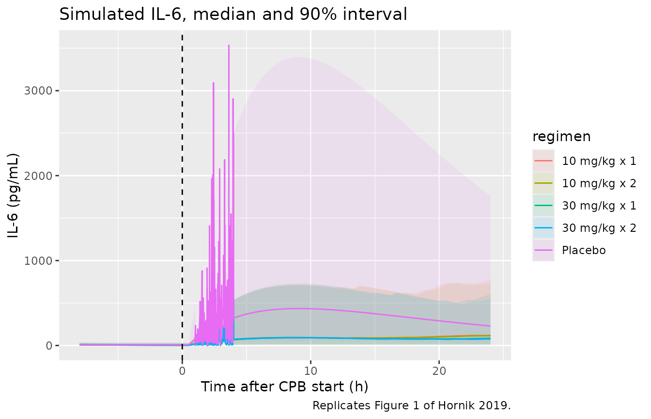
# Replicates Figure 2 of Hornik 2019: simulated IL-10 by regimen.
pi_plot(sim10, "il10", "IL-10 (pg/mL)", "Simulated IL-10, median and 90% interval") +
  labs(caption = "Replicates Figure 2 of Hornik 2019.")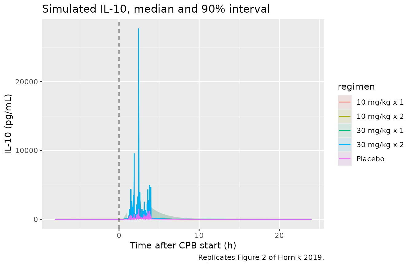
AUC0-24 after CPB start (Table 5, Tables S4-S5)
auc6 <- sim6 |>
  dplyr::group_by(base_id, regimen, RACHS1) |>
  dplyr::summarise(auc = auc_from_cpb(time, il6), .groups = "drop")
auc10 <- sim10 |>
  dplyr::group_by(base_id, regimen, PAGE) |>
  dplyr::summarise(auc = auc_from_cpb(time, il10), .groups = "drop")

paired_ratios <- function(auc) {
  w <- tidyr::pivot_wider(auc, names_from = regimen, values_from = auc)
  r <- list(
    `2 vs 1 dose` = c(w$`10 mg/kg x 2` / w$`10 mg/kg x 1`, w$`30 mg/kg x 2` / w$`30 mg/kg x 1`),
    `30 vs 10 mg/kg` = c(w$`30 mg/kg x 1` / w$`10 mg/kg x 1`, w$`30 mg/kg x 2` / w$`10 mg/kg x 2`),
    `10 mg/kg vs placebo` = c(w$`10 mg/kg x 1` / w$Placebo, w$`10 mg/kg x 2` / w$Placebo)
  )
  tibble::tibble(
    ratio = names(r),
    sim_mean = vapply(r, mean, 1),
    sim_median = vapply(r, median, 1)
  )
}
published_ratio <- tibble::tribble(
  ~ratio,                ~pub_il6, ~pub_il10,
  "2 vs 1 dose",         0.92,     1.08,
  "30 vs 10 mg/kg",      0.89,     1.03,
  "10 mg/kg vs placebo", 0.27,     3.85
)
r6 <- paired_ratios(auc6)
r10 <- paired_ratios(auc10)
ratio_tab <- published_ratio |>
  dplyr::left_join(dplyr::rename(r6, il6_mean = sim_mean, il6_median = sim_median), by = "ratio") |>
  dplyr::left_join(dplyr::rename(r10, il10_mean = sim_mean, il10_median = sim_median), by = "ratio")
ratio_tab |>
  dplyr::select(ratio, pub_il6, il6_mean, il6_median, pub_il10, il10_mean, il10_median) |>
  dplyr::rename(
    "Ratio" = ratio,
    "IL-6 Table 5 mean" = pub_il6,
    "IL-6 simulated mean" = il6_mean,
    "IL-6 simulated median" = il6_median,
    "IL-10 Table 5 mean" = pub_il10,
    "IL-10 simulated mean" = il10_mean,
    "IL-10 simulated median" = il10_median
  ) |>
knitr::kable(digits = 2, caption = "Paired AUC0-24 ratios versus Hornik 2019 Table 5.")| Ratio | IL-6 Table 5 mean | IL-6 simulated mean | IL-6 simulated median | IL-10 Table 5 mean | IL-10 simulated mean | IL-10 simulated median |
|---|---|---|---|---|---|---|
| 2 vs 1 dose | 0.92 | 0.96 | 0.97 | 1.08 | 1.01 | 1.01 |
| 30 vs 10 mg/kg | 0.89 | 0.89 | 0.87 | 1.03 | 1.01 | 1.01 |
| 10 mg/kg vs placebo | 0.27 | 0.27 | 0.25 | 3.85 | 4.26 | 3.12 |
The IL-6 ratios and the IL-10 dose-level and dose-number ratios reproduce Table 5 closely. The IL-10 methylprednisolone-versus-placebo ratio is a mean of per-subject ratios driven by the 110 %CV on Smax, so it is heavy-tailed and sensitive to the cohort. Its median sits below the published mean, as a right-skewed ratio’s median should.
s4 <- auc6 |>
  dplyr::mutate(RACHS = ifelse(RACHS1 >= 4, ">=4", "<4")) |>
  dplyr::group_by(RACHS, regimen) |>
  dplyr::summarise(sim_median = median(auc), .groups = "drop")
# Table S4 medians averaged over the three CPB-time strata, 1 dose rows
# (placebo 1-dose rows) -- RACHS-1 < 4: 30 mg/kg 909, 10 mg/kg 1010,
# placebo 3388; RACHS-1 >= 4: 30 mg/kg 2146, 10 mg/kg 2411, placebo 6572.
s4_pub <- tibble::tribble(
  ~RACHS, ~regimen,       ~pub_median,
  "<4",   "30 mg/kg x 1", mean(c(870, 910, 948)),
  "<4",   "10 mg/kg x 1", mean(c(988, 1004, 1037)),
  "<4",   "Placebo",      mean(c(3172, 3403, 3590)),
  ">=4",  "30 mg/kg x 1", mean(c(2056, 2136, 2246)),
  ">=4",  "10 mg/kg x 1", mean(c(2362, 2393, 2479)),
  ">=4",  "Placebo",      mean(c(6375, 6617, 6725))
)
s4_cmp <- dplyr::inner_join(s4_pub, s4, by = c("RACHS", "regimen")) |>
  dplyr::mutate(pct_diff = 100 * (sim_median / pub_median - 1))
s4_cmp |>
  dplyr::rename(
    "RACHS-1" = RACHS, "Regimen" = regimen,
    "Table S4 median" = pub_median, "Simulated median" = sim_median,
    "Difference (%)" = pct_diff
  ) |>
knitr::kable(digits = 0, caption = "IL-6 AUC0-24 (pg*h/mL) by RACHS-1 stratum versus Table S4.")| RACHS-1 | Regimen | Table S4 median | Simulated median | Difference (%) |
|---|---|---|---|---|
| <4 | 30 mg/kg x 1 | 909 | 1225 | 35 |
| <4 | 10 mg/kg x 1 | 1010 | 1377 | 36 |
| <4 | Placebo | 3388 | 5365 | 58 |
| >=4 | 30 mg/kg x 1 | 2146 | 2766 | 29 |
| >=4 | 10 mg/kg x 1 | 2411 | 3214 | 33 |
| >=4 | Placebo | 6572 | 11446 | 74 |
s5 <- auc10 |>
  dplyr::mutate(PMA = cut(PAGE, c(-Inf, 41, 42, Inf), labels = c("<=41", "41.1-42", ">42"))) |>
  dplyr::group_by(PMA, regimen) |>
  dplyr::summarise(sim_median = median(auc), .groups = "drop")
# Table S5 medians averaged over the three CPB-time strata, 1-dose rows.
s5_pub <- tibble::tribble(
  ~PMA,      ~regimen,       ~pub_median,
  "<=41",    "30 mg/kg x 1", mean(c(454, 698, 930)),
  "<=41",    "10 mg/kg x 1", mean(c(422, 674, 913)),
  "<=41",    "Placebo",      mean(c(165, 252, 337)),
  "41.1-42", "30 mg/kg x 1", mean(c(595, 943, 1255)),
  "41.1-42", "10 mg/kg x 1", mean(c(559, 903, 1227)),
  "41.1-42", "Placebo",      mean(c(222, 354, 475)),
  ">42",     "30 mg/kg x 1", mean(c(879, 1357, 1838)),
  ">42",     "10 mg/kg x 1", mean(c(835, 1306, 1783)),
  ">42",     "Placebo",      mean(c(339, 550, 754))
)
s5_cmp <- s5 |>
  dplyr::mutate(PMA = as.character(PMA)) |>
  dplyr::inner_join(s5_pub, by = c("PMA", "regimen")) |>
  dplyr::mutate(pct_diff = 100 * (sim_median / pub_median - 1))
s5_cmp |>
  dplyr::select(PMA, regimen, pub_median, sim_median, pct_diff) |>
  dplyr::rename(
    "PMA (weeks)" = PMA, "Regimen" = regimen,
    "Table S5 median" = pub_median, "Simulated median" = sim_median,
    "Difference (%)" = pct_diff
  ) |>
knitr::kable(digits = 0, caption = "IL-10 AUC0-24 (pg*h/mL) by PMA stratum versus Table S5.")| PMA (weeks) | Regimen | Table S5 median | Simulated median | Difference (%) |
|---|---|---|---|---|
| <=41 | 10 mg/kg x 1 | 670 | 569 | -15 |
| <=41 | 30 mg/kg x 1 | 694 | 590 | -15 |
| <=41 | Placebo | 251 | 158 | -37 |
| 41.1-42 | 10 mg/kg x 1 | 896 | 867 | -3 |
| 41.1-42 | 30 mg/kg x 1 | 931 | 887 | -5 |
| 41.1-42 | Placebo | 350 | 339 | -3 |
| >42 | 10 mg/kg x 1 | 1308 | 1529 | 17 |
| >42 | 30 mg/kg x 1 | 1358 | 1606 | 18 |
| >42 | Placebo | 548 | 451 | -18 |
Most IL-10 stratum medians fall within about 20% of Table S5. The
least-mature placebo stratum is lower, which the uniform-PNA cohort (PMA
40-41 weeks within that stratum) and the steep PMA exponent of 14.8
explain. The IL-6 medians run 30-75% above Table S4, placebo rows most.
The gap is already present for the typical subject: RACHS-1 below 4,
156.5 min bypass, placebo gives 4341 pg*h/mL against about 3400 in the
120-180 min row of Table S4. Yet the IL-6 regimen ratios reproduce Table
5. A difference that scales every IL-6 exposure about equally points to
how the paper’s NONMEM simulation evaluated the CPB time course, not to
a transcription error. The CPB effect enters every regimen, placebo
included, while the drug parameters would move the ratios. NONMEM
evaluates $PK quantities such as CPBV,
CPBES and the withdrawal term
EXP(-0.693*TACPB/CPBH) once per data record, so they are
piecewise constant over the simulation grid. The simulation data set is
not published, so this cannot be checked. The parameters are not
adjusted to close the gap.
stopifnot(
  # Structural: a wrong IC50 unit, Hill or CPB term moves these by far more.
  abs(r6$sim_mean[r6$ratio == "10 mg/kg vs placebo"] / 0.27 - 1) < 0.25,
  abs(r6$sim_mean[r6$ratio == "30 vs 10 mg/kg"] / 0.89 - 1) < 0.10,
  abs(r10$sim_median[r10$ratio == "30 vs 10 mg/kg"] / 1.03 - 1) < 0.10,
  r10$sim_median[r10$ratio == "10 mg/kg vs placebo"] > 2,
  # IL-10 strata: centre and envelope (each median has ~15% Monte-Carlo SE).
  abs(median(s5_cmp$pct_diff)) < 25,
  quantile(abs(s5_cmp$pct_diff), 0.9) < 50,
  # IL-6 strata: the documented level gap above, bounded at a factor of 2.5
  # per row so that a mis-transcribed CPBE or baseline (a multi-fold shift)
  # still fails.
  all(abs(log(s4_cmp$sim_median / s4_cmp$pub_median)) < log(2.5))
)
PKNCA validation of the methylprednisolone PK
The paper reports no NCA, but it states typical values for a 3.2 kg neonate (CL/F 3.88 L/h, Table 2; the Discussion rounds to 3.8 L/h) and median post hoc clearances of 1.28 L/h/kg before CPB and 1.24 L/h/kg after CPB. For a typical 3.2 kg neonate with a 156.5 min bypass, pre- and post-CPB clearance are identical, so the PKNCA clearance from a single 30 mg/kg dose must return 3.88 L/h. The half-life should match the slower eigenvalue of the two-compartment system.
ev_pk <- make_subject_events(1, 30, 1, WT = 3.2, T_CPB = 156.5, obs_cmt = "il6") |>
  dplyr::mutate(RACHS1 = 3)
grid_long <- sort(unique(c(ev_pk$time[ev_pk$evid == 0], seq(32, 400, by = 2))))
ev_pk <- dplyr::bind_rows(
  ev_pk,
  data.frame(id = 1, time = setdiff(grid_long, ev_pk$time), evid = 0, amt = 0, rate = 0, cmt = "il6") |>
    dplyr::mutate(WT = 3.2, T_CPB = 156.5, CPB_ON = 0, CPB_POST = 1, RACHS1 = 3)
) |>
  dplyr::arrange(time, dplyr::desc(evid))
ev_pk$treatment <- "30 mg/kg x 1"
sim_pk <- as.data.frame(rxode2::rxSolve(typ6, ev_pk,
  returnType = "data.frame", rtol = 1e-10, atol = 1e-12
))
#> ℹ omega/sigma items treated as zero: 'etalcl', 'etalvc', 'etalq', 'etalrbase', 'etalcpbe'
sim_pk$treatment <- "30 mg/kg x 1"
sim_pk$id <- 1L # a single-subject solve returns no id column

conc_pk <- sim_pk |>
  dplyr::filter(!is.na(Cc)) |>
  dplyr::mutate(time = time - t_cpb_start, conc = pmax(Cc, 0) / 1000) |>
  dplyr::filter(time >= 0) |>
  dplyr::select(id, time, conc, treatment)
conc_pk <- dplyr::bind_rows(conc_pk, dplyr::distinct(conc_pk, id, treatment) |> dplyr::mutate(time = 0, conc = 0)) |>
  dplyr::distinct(id, treatment, time, .keep_all = TRUE) |>
  dplyr::arrange(id, time)
dose_pk <- ev_pk |>
  dplyr::filter(evid == 1) |>
  dplyr::mutate(time = time - t_cpb_start) |>
  dplyr::select(id, time, amt, treatment)

nca_pk <- PKNCA::pk.nca(PKNCA::PKNCAdata(
  PKNCA::PKNCAconc(conc_pk, conc ~ time | treatment + id),
  PKNCA::PKNCAdose(dose_pk, amt ~ time | treatment + id),
  intervals = data.frame(start = 0, end = Inf, cmax = TRUE, tmax = TRUE,
                         aucinf.obs = TRUE, half.life = TRUE, cl.obs = TRUE)
))

vc <- 8.92; vp <- 16.81; cl <- 3.88; q <- 0.10
k10 <- cl / vc; k12 <- q / vc; k21 <- q / vp
beta <- ((k10 + k12 + k21) - sqrt((k10 + k12 + k21)^2 - 4 * k10 * k21)) / 2
published_pk <- tibble::tibble(treatment = "30 mg/kg x 1", cl.obs = 3.88, half.life = log(2) / beta)
cmp_pk <- nlmixr2lib::ncaComparisonTable(
  simulated = nca_pk,
  reference = published_pk,
  by = "treatment",
  units = c(cl.obs = "L/h", half.life = "h"),
  tolerance_pct = 20
)
knitr::kable(cmp_pk, caption = "Typical 3.2 kg neonate: PKNCA versus Table 2 CL and the model's terminal half-life. * differs by >20%.")| NCA parameter | treatment | Reference | Simulated | % diff |
|---|---|---|---|---|
| t½ (h) | 30 mg/kg x 1 | 120 | 119 | -0.2% |
| CL/F (L/h) | 30 mg/kg x 1 | 3.88 | 3.88 | +0.0% |
nca_tab <- as.data.frame(nca_pk$result)
stopifnot(
  abs(nca_tab$PPORRES[nca_tab$PPTESTCD == "cl.obs"] / 3.88 - 1) < 0.02,
  abs(nca_tab$PPORRES[nca_tab$PPTESTCD == "half.life"] / (log(2) / beta) - 1) < 0.10
)
The long terminal half-life (120 h) follows from the small intercompartmental clearance (Q = 0.10 L/h) against a large peripheral volume. It is a property of the published parameters and is invisible over the study’s 24 h post-CPB sampling window.
Per-kilogram individual clearance in the stochastic IL-6 cohort, 30 mg/kg single-dose regimen, compared with the paper’s median post hoc estimates:
cl_kg <- sim6 |>
  dplyr::filter(regimen == "30 mg/kg x 1") |>
  dplyr::mutate(phase = ifelse(time < t_cpb_start, "pre-CPB", ifelse(time > t_cpb_start + 4.5, "post-CPB", NA))) |>
  dplyr::filter(!is.na(phase)) |>
  dplyr::group_by(base_id, phase) |>
  dplyr::summarise(cl_kg = dplyr::first(cl) / dplyr::first(WT), .groups = "drop") |>
  dplyr::group_by(phase) |>
  dplyr::summarise(sim_median = median(cl_kg), .groups = "drop") |>
  dplyr::left_join(tibble::tibble(phase = c("pre-CPB", "post-CPB"), published = c(1.28, 1.24)), by = "phase")
cl_kg |>
  dplyr::rename("Phase" = phase, "Simulated median (L/h/kg)" = sim_median, "Published EBE median (L/h/kg)" = published) |>
knitr::kable(digits = 2)| Phase | Simulated median (L/h/kg) | Published EBE median (L/h/kg) |
|---|---|---|
| post-CPB | 1.23 | 1.24 |
| pre-CPB | 1.18 | 1.28 |
Assumptions and deviations
-
CPB timing encoded as time-varying indicators. The
control streams derive the CPB windows from a sample index
(
POINT) and aCPBSTARTdata column. HereCPB_ONandCPB_POSTare data columns and the 0.5 h onset delay (CPBES) and post-CPB withdrawal of the IL-6 CPB effect are computed inside the model from two bookkeeping states (cpb_elapsed,cpb_decay), which reproduces Eq. 6 exactly in continuous time. -
POSTCPB. The control streams code the clearance
switch as
STA4 = STA2 + STA3, whose flag definitions are not given. The paper names the indicator POSTCPB (“time after CPB”) and reports pre- versus post-CPB clearance, so it is encoded asCPB_POST. - PK values. The PD control streams (Data S1, S2) carry PK thetas that differ from Table 2 (V2 8.848, V3 11.58, Q 0.0868 versus 8.92, 16.81, 0.10). The PD fits used individual PK estimates, so these thetas did not drive the PD. The published final estimates in Table 2 are used. The Discussion’s Vss/F of 26.3 L is closer to Table 2 (Vc + Vp = 25.7 L) than to the stream values (20.4 L).
-
IIV scale. Tables 2-4 report IIV as %CV only, and
the control-stream
$OMEGAinitials are not near-converged, so they cannot settle the scale. The library convention omega^2 = log(1 + CV^2) is used. For the large IL-6 and IL-10 PD variabilities (83.6-110 %CV) the alternative reading omega^2 = CV^2 would give wider distributions. -
Residual error. NONMEM
Y = EFF*EXP(ERR(1))under FOCE-I is linearised to a proportional error, and the paper reports it as “Proportional error, %”. It is encoded asprop()with SD = %/100. -
PD driver units. The streams use
A(2)/V2(mg/L) inside$DES, while the paper reports IC50 and SC50 in ng/mL. The model uses the ng/mLCc, and the typical-value check above shows this is the only reading that reproduces Table 5. - Dosing route. As in the paper, every prodrug dose (including a dose into the CPB circuit) enters one depot and converts completely to methylprednisolone at rate Kf, with no prodrug renal clearance (Discussion, limitations).
- IL-6 absolute exposure versus Table S4. Simulated IL-6 AUC0-24 medians are 30-75% higher than Table S4 in every stratum, while the Table 5 regimen ratios, the IL-10 Table S5 medians and the PK typical values reproduce. The model is not adjusted; see the discussion under the AUC tables for the likely cause (record-wise evaluation of the CPB time course in the paper’s NONMEM simulation).
- Virtual population. The PK-Sim cohort of the paper (1,000 term infants, 50% female, 85% White) is replaced by the simple normal-weight, uniform-PNA cohort above. The Table S4/S5 comparison is therefore approximate; the paired ratios in Table 5 depend much less on the covariate distribution.