BTK occupancy by zanubrutinib, acalabrutinib and ibrutinib (Demin 2025)
Source:vignettes/articles/Demin_2025_zanubrutinib_acalabrutinib_ibrutinib_qsp.Rmd
Demin_2025_zanubrutinib_acalabrutinib_ibrutinib_qsp.RmdThe model
Demin and colleagues built a quantitative systems pharmacology (QSP) model to explain why three approved covalent Bruton tyrosine kinase (BTK) inhibitors – zanubrutinib, acalabrutinib and ibrutinib – give different progression-free survival despite similar-looking trough BTK occupancy. The model chains four layers together:
- a two-compartment population-PK model for each moiety (the two parent drugs plus the active metabolites ACP-5862 and PCI-45227, and zanubrutinib which has none);
- perfusion-limited transport of unbound drug from plasma into the interstitial fluid (ISF) of lymph nodes (LN) and bone marrow (BM);
- an equilibrium partition from ISF (or from plasma, for PBMCs) into the intracellular space of CLL cells; and
- an ATP-competitive, covalently inactivating BTK-binding module sitting on top of BTK synthesis and degradation.
Because all five moieties compete for the same BTK pool in each tissue, this is one coupled system rather than three separate models, and it is packaged as a single model file.
mod <- rxode2::rxode(readModelDb("Demin_2025_zanubrutinib_acalabrutinib_ibrutinib_qsp"))
#> ℹ parameter labels from comments will be replaced by 'label()'
#> Warning: some etas defaulted to non-mu referenced, possible parsing error: etaiovlvc_zan, etaiovlcl_zan, etaiovlcl_ibr, etaiovlcl_pci
#> as a work-around try putting the mu-referenced expression on a simple line
length(mod$state)
#> [1] 67
The 67 ODE states break down as 21 PK states (gut / transit / depot / central / peripheral for each moiety), 10 ISF states (5 moieties x 2 tissues) and 36 BTK states (3 tissues x {free BTK, BTK:ATP, and a bound plus an inactivated species for each of the 5 moieties}).
Population
The source is a simulation study rather than a fit to individual data. The authors generated 1000 virtual patients by sampling the parameter distributions in Table S1, and validated the predictions against published BTK-occupancy data from patients with chronic lymphocytic leukaemia (CLL). The BTK-binding module is parameterised for primary CLL cells.
str(mod$population, max.level = 1)
#> List of 5
#>  $ species      : chr "human"
#>  $ n_subjects   : int 1000
#>  $ disease_state: chr "B-cell malignancies (chronic lymphocytic leukaemia / small lymphocytic lymphoma, mantle cell lymphoma and Walde"| __truncated__
#>  $ dose_range   : chr "Zanubrutinib 160 mg BID or 320 mg QD (reduced doses 80 mg BID, 80 mg QD); acalabrutinib 100 mg BID, 100 mg QD o"| __truncated__
#>  $ notes        : chr "In silico cohort: 1000 virtual patients generated by sampling the parameter distributions in Table S1 (Methods "| __truncated__
The underlying PK parameters are not fitted here – they are taken from previously published population-PK analyses and reproduced in Table S1 of the source: zanubrutinib from Ou 2021 (PMID 33306268), acalabrutinib and ACP-5862 from Edlund 2022 (PMID 34265100) with ACP-5862 disposition from Edlund 2019 (PMID 30556110), and ibrutinib with PCI-45227 from Gallais 2020 (PMID 32328976).
Source trace
Every value in ini() carries an in-file comment pointing
at its origin. The table below is the vignette-level summary; the model
file is the line-by-line audit trail.
| Model component | Source location |
|---|---|
Perfusion-limited ISF transport (d/dt(isf_*)) |
Supplement equation 1 |
ISF-to-intracellular partition (ccell_*) |
Supplement equation 2 |
Free BTK balance (d/dt(btk_free_*)) |
Supplement equation 3 |
BTK:ATP complex (d/dt(btk_atp_*)) |
Supplement equation 4 |
BTK:inhibitor complex (d/dt(btk_<drug>_*)) |
Supplement equation 5 |
Inactivated BTK (d/dt(btk_<drug>_inact_*)) |
Supplement equation 6 |
BTK synthesis vsyn = bl_btk * kdeg
|
Supplement equation 7 |
Intracellular partition coefficient kp_cell
|
Supplement equation 8 |
Erythrocyte-to-plasma coefficient kp_rbc
|
Supplement equation 9 (Hinderling 1997) |
kd_<drug> from IC50 ratios |
Supplement equation 10 |
| All PK parameters and their IIV / IOV | Table S1, “PK parameters” |
All binding parameters (koff, kd,
kinact, bp, fup) |
Table S1, “Drug-specific non-PK parameters” |
q_ln, q_bm, bl_btk,
koff_atp, kd_atp, c_adj_pbmc
|
Table S1, “Systemic parameters” |
ISF volumes v_isf_ln, v_isf_bm
|
Model code Compartment sheet (LN_isf,
BM_isf) |
Molecular weights mr_*, unit conversions |
Model code Const sheet |
The executable Heta-compiler model shipped as Supporting Information (“Model_Code/src/BTKi_PK_TO.xlsx”) was used as the authoritative source for the rate laws and for the handful of values where it disagrees with Table S1; those disagreements are listed under Assumptions and deviations below.
Structural check: BTK mass balance
The BTK module has an exact invariant that is worth checking before
any occupancy number is trusted. Synthesis is
vsyn = bl_btk * kdeg, and every BTK species (free,
ATP-bound, inhibitor-bound and inactivated) degrades with the same
first-order constant kdeg. Therefore
d(total BTK)/dt = bl_btk * kdeg - kdeg * total BTK = kdeg * (bl_btk - total BTK)so total BTK started at bl_btk must stay at
bl_btk for all time, in every tissue, under any dosing
regimen. This is a strong test: it exercises the synthesis term, all 12
degradation terms per tissue and the binding / inactivation bookkeeping
simultaneously, and any sign or index error breaks it.
typical <- zeroRe(mod)
#> Warning: No sigma parameters in the model
#> Warning: some etas defaulted to non-mu referenced, possible parsing error: etaiovlvc_zan, etaiovlcl_zan, etaiovlcl_ibr, etaiovlcl_pci
#> as a work-around try putting the mu-referenced expression on a simple line

ev_mb <-
  et(amt = 160, cmt = "gut_zan", ii = 0.5, until = 10) %>%
  et(seq(0, 12, by = 0.25))

mb <- rxSolve(typical, ev_mb, atol = 1e-10, rtol = 1e-8)
#> ℹ omega/sigma items treated as zero: 'etald1_zan', 'etalvc_zan', 'etalvp_zan', 'etalcl_zan', 'etalq_zan', 'etalvc_aca', 'etalcl_aca', 'etalvc_acp', 'etalvp_acp', 'etalcl_acp', 'etalq_acp', 'etald1_ibr', 'etalvc_ibr', 'etalvp_ibr', 'etalcl_ibr', 'etalkabs_pci', 'etalclmet_ibr', 'etalcl_pci', 'etalatp', 'etalkdeg_btk', 'etaiovlvc_zan', 'etaiovlcl_zan', 'etaiovlmtt_aca', 'etaiovlf1_aca', 'etaiovlcl_ibr', 'etaiovlcl_pci'

# baseline read from the model, not hard-coded, so this cannot pass against a
# stale literal
bl_btk <- mod$theta[["bl_btk"]]

mass_balance <- tibble::tibble(
  Tissue = c("PBMC", "Lymph node", "Bone marrow"),
  `Max abs. deviation from baseline (nmol/L)` = c(
    max(abs(mb$btk_total_pbmc - bl_btk)),
    max(abs(mb$btk_total_ln - bl_btk)),
    max(abs(mb$btk_total_bm - bl_btk))
  )
)
knitr::kable(mass_balance, digits = 10)| Tissue | Max abs. deviation from baseline (nmol/L) |
|---|---|
| PBMC | 1e-10 |
| Lymph node | 1e-10 |
| Bone marrow | 1e-10 |
# the check must be able to fail the render, not merely be printed
stopifnot(all(mass_balance[[2]] < 1e-6))
Total BTK is conserved at the baseline 561.3 nmol/L (the value of
bl_btk) to solver tolerance in all three tissues, as
required.
Plasma pharmacokinetics
The PK layer reproduces the published population-PK models. The source plots these profiles in Figure S1 but tabulates no NCA summary statistics, so there is no published NCA table to compare against. Instead the PK layer is checked against an exact closed-form identity that it must satisfy at steady state (below), with the NCA output reported descriptively.
arms <- tibble::tribble(
  ~arm,                       ~cmt,       ~dose, ~ii,
  "Zanubrutinib 160 mg BID",  "gut_zan",  160,   0.5,
  "Acalabrutinib 100 mg BID", "gut_aca",  100,   0.5,
  "Ibrutinib 420 mg QD",      "gut_ibr",  420,   1.0
)

parent_conc <- c(gut_zan = "Cc_zan", gut_aca = "Cc_aca", gut_ibr = "Cc_ibr")

LAST_DOSE <- 14  # days; PK and occupancy are at steady state well before this

# Dose to steady state, then observe the dosing interval that follows the last
# dose, so the profile covers a full interval rather than ending at it.
pk <- lapply(seq_len(nrow(arms)), function(i) {
  ii <- arms$ii[i]
  ev <-
    et(amt = arms$dose[i], cmt = arms$cmt[i], ii = ii, until = LAST_DOSE) %>%
    et(seq(LAST_DOSE, LAST_DOSE + ii, by = 0.002))
  s <- rxSolve(typical, ev, atol = 1e-10, rtol = 1e-8)
  tibble::tibble(
    arm   = arms$arm[i],
    tad_h = (s$time - LAST_DOSE) * 24,
    conc  = s[[parent_conc[[arms$cmt[i]]]]]
  )
}) %>%
  dplyr::bind_rows()
#> ℹ omega/sigma items treated as zero: 'etald1_zan', 'etalvc_zan', 'etalvp_zan', 'etalcl_zan', 'etalq_zan', 'etalvc_aca', 'etalcl_aca', 'etalvc_acp', 'etalvp_acp', 'etalcl_acp', 'etalq_acp', 'etald1_ibr', 'etalvc_ibr', 'etalvp_ibr', 'etalcl_ibr', 'etalkabs_pci', 'etalclmet_ibr', 'etalcl_pci', 'etalatp', 'etalkdeg_btk', 'etaiovlvc_zan', 'etaiovlcl_zan', 'etaiovlmtt_aca', 'etaiovlf1_aca', 'etaiovlcl_ibr', 'etaiovlcl_pci'
#> ℹ omega/sigma items treated as zero: 'etald1_zan', 'etalvc_zan', 'etalvp_zan', 'etalcl_zan', 'etalq_zan', 'etalvc_aca', 'etalcl_aca', 'etalvc_acp', 'etalvp_acp', 'etalcl_acp', 'etalq_acp', 'etald1_ibr', 'etalvc_ibr', 'etalvp_ibr', 'etalcl_ibr', 'etalkabs_pci', 'etalclmet_ibr', 'etalcl_pci', 'etalatp', 'etalkdeg_btk', 'etaiovlvc_zan', 'etaiovlcl_zan', 'etaiovlmtt_aca', 'etaiovlf1_aca', 'etaiovlcl_ibr', 'etaiovlcl_pci'
#> ℹ omega/sigma items treated as zero: 'etald1_zan', 'etalvc_zan', 'etalvp_zan', 'etalcl_zan', 'etalq_zan', 'etalvc_aca', 'etalcl_aca', 'etalvc_acp', 'etalvp_acp', 'etalcl_acp', 'etalq_acp', 'etald1_ibr', 'etalvc_ibr', 'etalvp_ibr', 'etalcl_ibr', 'etalkabs_pci', 'etalclmet_ibr', 'etalcl_pci', 'etalatp', 'etalkdeg_btk', 'etaiovlvc_zan', 'etaiovlcl_zan', 'etaiovlmtt_aca', 'etaiovlf1_aca', 'etaiovlcl_ibr', 'etaiovlcl_pci'

ggplot(pk, aes(tad_h, conc, colour = arm)) +
  geom_line(linewidth = 0.8) +
  scale_y_log10() +
  labs(x = "Time after dose (h)", y = "Plasma concentration (ng/mL)",
       colour = NULL) +
  theme_bw() +
  theme(legend.position = "bottom")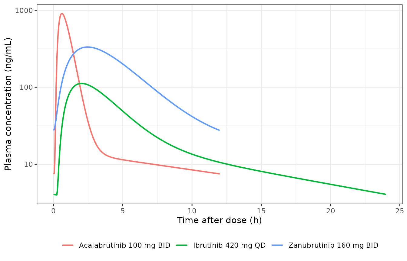
Typical-value plasma concentration-time profiles over one steady-state dosing interval. Compare with Figure S1 of Demin 2025.
nca_input <- pk %>%
  dplyr::filter(!is.na(conc)) %>%
  dplyr::mutate(id = 1L) %>%
  as.data.frame()

dose_input <- arms %>%
  dplyr::transmute(arm, id = 1L, tad_h = 0, dose) %>%
  as.data.frame()

conc_obj <- PKNCA::PKNCAconc(nca_input, conc ~ tad_h | arm + id,
                             concu = "ng/mL", timeu = "h")
dose_obj <- PKNCA::PKNCAdose(dose_input, dose ~ tad_h | arm + id,
                             doseu = "mg")

intervals <- arms %>%
  dplyr::transmute(
    start = 0, end = ii * 24, arm, id = 1L,
    cmax = TRUE, tmax = TRUE, auclast = TRUE, half.life = TRUE
  ) %>%
  as.data.frame()

nca <- PKNCA::pk.nca(PKNCA::PKNCAdata(conc_obj, dose_obj, intervals = intervals))

nca_tab <- as.data.frame(nca) %>%
  dplyr::filter(PPTESTCD %in% c("cmax", "tmax", "auclast", "half.life")) %>%
  tidyr::pivot_wider(id_cols = arm, names_from = PPTESTCD, values_from = PPORRES)

nca_tab %>%
  dplyr::rename(
    "Regimen" = arm,
    "Cmax (ng/mL)" = cmax,
    "Tmax (h)" = tmax,
    "AUCtau (ng*h/mL)" = auclast,
    "Apparent half-life over tau (h)" = half.life
  ) %>%
  knitr::kable(digits = 2,
caption = "Steady-state NCA of the typical-value profiles over one dosing interval.")| Regimen | AUCtau (ng*h/mL) | Cmax (ng/mL) | Tmax (h) | Apparent half-life over tau (h) |
|---|---|---|---|---|
| Zanubrutinib 160 mg BID | 1791.63 | 333.31 | 2.45 | 4.09 |
| Acalabrutinib 100 mg BID | 979.31 | 908.63 | 0.62 | 11.51 |
| Ibrutinib 420 mg QD | 603.40 | 112.16 | 2.02 | 9.09 |
Simulated Tmax reproduces the known absorption behaviour of the three drugs (acalabrutinib fastest at about 0.6 h, zanubrutinib and ibrutinib around 2-2.5 h). The half-life column is deliberately not compared against the 2-4 h / 0.6-2.8 h / 4-6 h mean plasma half-lives quoted in the paper’s Introduction: those are effective half-lives, whereas a log-linear slope fitted inside a single dosing interval of a two-compartment model estimates neither the distribution nor the true terminal phase. Reading it as a pass/fail check would be an apples-to-oranges comparison.
Closed-form exposure check
The steady-state exposure of this model is fixed by mass balance and does not depend on the volumes, the inter-compartmental clearance or the absorption rate constants. For each parent moiety,
AUC_tau = (fraction of dose reaching the central compartment) x dose / CL_totalFor zanubrutinib and acalabrutinib the whole dose reaches central and
CL_total is cl_zan / cl_aca (for
acalabrutinib both the Fm and the 1 - Fm
branch are driven by cl_aca, so the metabolite split does
not change parent exposure). For ibrutinib the depot feeds two parallel
first-order paths – kabs_ibr to ibrutinib and
kabs_pci straight to PCI-45227 – so only
kabs_ibr / (kabs_ibr + kabs_pci) of the dose ever appears
as ibrutinib, and its total elimination is
cl_ibr + clmet_ibr. This is an independent check on the
clearance parameters, the metabolite branching and the unit conversions
all at once.
th <- mod$theta

kabs_ibr  <- th[["kabs_ibr"]]
kabs_pci  <- exp(th[["lkabs_pci"]])
f_to_ibr  <- kabs_ibr / (kabs_ibr + kabs_pci)

expected_auc <- c(
  "Zanubrutinib 160 mg BID"  = 160 / exp(th[["lcl_zan"]]),
  "Acalabrutinib 100 mg BID" = 100 / exp(th[["lcl_aca"]]),
  "Ibrutinib 420 mg QD"      =
    420 * f_to_ibr / (exp(th[["lcl_ibr"]]) + exp(th[["lclmet_ibr"]]))
)
# mg*day/L -> ng*h/mL
expected_auc <- expected_auc * 1000 * 24

auc_check <- nca_tab %>%
  dplyr::transmute(
    arm,
    simulated = auclast,
    expected  = unname(expected_auc[arm]),
    `relative difference (%)` = 100 * (auclast - expected) / expected
  )

auc_check %>%
  dplyr::rename("Regimen" = arm, "Simulated AUCtau" = simulated,
                "Closed-form AUCtau" = expected) %>%
  knitr::kable(digits = c(0, 1, 1, 4),
caption = "Steady-state AUC over one dosing interval (ng*h/mL): simulated versus the closed-form dose / clearance identity.")| Regimen | Simulated AUCtau | Closed-form AUCtau | relative difference (%) |
|---|---|---|---|
| Zanubrutinib 160 mg BID | 1791.6 | 1791.7 | -0.0049 |
| Acalabrutinib 100 mg BID | 979.3 | 979.6 | -0.0287 |
| Ibrutinib 420 mg QD | 603.4 | 603.4 | -0.0010 |
All three arms agree with the closed form to well under 0.5%, confirming the clearance parameters, the ibrutinib pre-systemic metabolite branch and the mg/L-to-ng/mL conversion.
BTK occupancy at steady state
The virtual cohort is capped at 200 subjects per arm in this vignette (the source used 1000), so every percentage below carries a binomial Monte Carlo error of roughly 1-4 percentage points.
N_SUB <- 200L

sim_cohort <- function(cmt, dose, ii, times, n = N_SUB, seed = 20250815) {
  set.seed(seed)
  ev <-
    et(amt = dose, cmt = cmt, ii = ii, until = LAST_DOSE) %>%
    et(times)
  rxSolve(mod, ev, nSub = n, atol = 1e-9, rtol = 1e-7, maxsteps = 100000L)
}

obs_times <- c(LAST_DOSE, LAST_DOSE + 1, LAST_DOSE + 2, LAST_DOSE + 3)

cohort <- lapply(seq_len(nrow(arms)), function(i) {
  s <- sim_cohort(arms$cmt[i], arms$dose[i], arms$ii[i], obs_times)
  tibble::tibble(
    arm  = arms$arm[i],
    id   = s$sim.id,
    time = s$time,
    hours_after_last_dose = round((s$time - LAST_DOSE) * 24),
    PBMC = s$occupancy_pbmc,
    LN   = s$occupancy_ln,
    BM   = s$occupancy_bm
  )
}) %>%
  dplyr::bind_rows()

# no subject was lost to a failed solve
stopifnot(nrow(cohort) == nrow(arms) * N_SUB * length(obs_times),
          !anyNA(cohort$PBMC), !anyNA(cohort$LN), !anyNA(cohort$BM))
Median trough occupancy versus observed data (Table S2)
Table S2 of the source lists observed median trough BTK occupancy with the range excluding outliers.
observed_s2 <- tibble::tribble(
  ~arm,                       ~tissue, ~observed,
  "Zanubrutinib 160 mg BID",  "PBMC",  "100 (99.2-100)",
  "Zanubrutinib 160 mg BID",  "LN",    "100 (97.2-100)",
  "Acalabrutinib 100 mg BID", "PBMC",  "95.3 (92.3-98.5)",
  "Acalabrutinib 100 mg BID", "LN",    "97.6 (94.5-99.2)",
  "Ibrutinib 420 mg QD",      "PBMC",  "89.3 (83.8-95.7) / 97.4 (88-100)",
  "Ibrutinib 420 mg QD",      "LN",    "97.5 (88.9-100)"
)

trough <- cohort %>% dplyr::filter(hours_after_last_dose == 0)

simulated_s2 <- trough %>%
  tidyr::pivot_longer(c(PBMC, LN, BM), names_to = "tissue",
                      values_to = "occ") %>%
  dplyr::filter(tissue %in% c("PBMC", "LN")) %>%
  dplyr::group_by(arm, tissue) %>%
  dplyr::summarise(
    simulated = sprintf("%.1f (%.1f-%.1f)", median(occ),
                        quantile(occ, 0.025), quantile(occ, 0.975)),
    .groups = "drop"
  )

observed_s2 %>%
  dplyr::left_join(simulated_s2, by = c("arm", "tissue")) %>%
  dplyr::rename(
    "Regimen" = arm,
    "Tissue" = tissue,
    "Observed median (range)" = observed,
    "Simulated median (95% CI)" = simulated
  ) %>%
knitr::kable(caption = "Trough BTK occupancy at steady state. Observed values are Table S2 of Demin 2025; the two ibrutinib PBMC entries are treatment-naive and relapsed/refractory CLL cohorts respectively. Replicates Figure 2 of Demin 2025.")| Regimen | Tissue | Observed median (range) | Simulated median (95% CI) |
|---|---|---|---|
| Zanubrutinib 160 mg BID | PBMC | 100 (99.2-100) | 99.0 (94.5-99.8) |
| Zanubrutinib 160 mg BID | LN | 100 (97.2-100) | 99.2 (95.7-99.8) |
| Acalabrutinib 100 mg BID | PBMC | 95.3 (92.3-98.5) | 95.3 (86.3-99.1) |
| Acalabrutinib 100 mg BID | LN | 97.6 (94.5-99.2) | 96.3 (89.2-99.3) |
| Ibrutinib 420 mg QD | PBMC | 89.3 (83.8-95.7) / 97.4 (88-100) | 96.4 (73.3-99.3) |
| Ibrutinib 420 mg QD | LN | 97.5 (88.9-100) | 97.2 (78.4-99.5) |
Percentage of patients above the occupancy thresholds (Table 1 and Table S3)
This is the paper’s headline quantitative result. z is
the difference between the simulated and published percentage expressed
in units of the binomial Monte Carlo standard error of a 200-subject
cohort, so values within about |z| < 2 are consistent
with the published 1000-subject numbers.
published_trough <- tibble::tribble(
  ~arm,                       ~tissue, ~pub95, ~pub90,
  "Zanubrutinib 160 mg BID",  "PBMC",  93.7,   99.3,
  "Zanubrutinib 160 mg BID",  "LN",    97.2,   99.6,
  "Zanubrutinib 160 mg BID",  "BM",    99.6,   99.9,
  "Acalabrutinib 100 mg BID", "PBMC",  55.2,   89.7,
  "Acalabrutinib 100 mg BID", "LN",    68.9,   95.3,
  "Acalabrutinib 100 mg BID", "BM",    93.0,   99.6,
  "Ibrutinib 420 mg QD",      "PBMC",  64.9,   86.9,
  "Ibrutinib 420 mg QD",      "LN",    74.3,   91.6,
  "Ibrutinib 420 mg QD",      "BM",    89.3,   98.2
)

mc_se <- function(p, n = N_SUB) 100 * sqrt((p / 100) * (1 - p / 100) / n)

trough %>%
  tidyr::pivot_longer(c(PBMC, LN, BM), names_to = "tissue",
                      values_to = "occ") %>%
  dplyr::group_by(arm, tissue) %>%
  dplyr::summarise(sim95 = 100 * mean(occ > 95),
                   sim90 = 100 * mean(occ > 90), .groups = "drop") %>%
  dplyr::left_join(published_trough, by = c("arm", "tissue")) %>%
  dplyr::mutate(z95 = (sim95 - pub95) / mc_se(pub95),
                z90 = (sim90 - pub90) / mc_se(pub90)) %>%
  dplyr::select(arm, tissue, sim95, pub95, z95, sim90, pub90, z90) %>%
  dplyr::rename(
    "Regimen" = arm, "Tissue" = tissue,
    "Simulated >95%" = sim95, "Published >95%" = pub95, "z (95%)" = z95,
    "Simulated >90%" = sim90, "Published >90%" = pub90, "z (90%)" = z90
  ) %>%
  knitr::kable(digits = 1,
caption = "Percentage of patients with trough BTK occupancy above 95% (Table 1 of Demin 2025) and above 90% (Table S3).")| Regimen | Tissue | Simulated >95% | Published >95% | z (95%) | Simulated >90% | Published >90% | z (90%) |
|---|---|---|---|---|---|---|---|
| Acalabrutinib 100 mg BID | BM | 95.0 | 93.0 | 1.1 | 100.0 | 99.6 | 0.9 |
| Acalabrutinib 100 mg BID | LN | 73.0 | 68.9 | 1.3 | 96.5 | 95.3 | 0.8 |
| Acalabrutinib 100 mg BID | PBMC | 53.5 | 55.2 | -0.5 | 91.5 | 89.7 | 0.8 |
| Ibrutinib 420 mg QD | BM | 85.0 | 89.3 | -2.0 | 95.0 | 98.2 | -3.4 |
| Ibrutinib 420 mg QD | LN | 70.5 | 74.3 | -1.2 | 87.0 | 91.6 | -2.3 |
| Ibrutinib 420 mg QD | PBMC | 63.0 | 64.9 | -0.6 | 84.0 | 86.9 | -1.2 |
| Zanubrutinib 160 mg BID | BM | 100.0 | 99.6 | 0.9 | 100.0 | 99.9 | 0.4 |
| Zanubrutinib 160 mg BID | LN | 98.0 | 97.2 | 0.7 | 100.0 | 99.6 | 0.9 |
| Zanubrutinib 160 mg BID | PBMC | 96.5 | 93.7 | 1.6 | 100.0 | 99.3 | 1.2 |
Occupancy after dose interruption (Table 1 and Table S4)
The paper’s central clinical message is that the three inhibitors
separate much more sharply after a missed dose than at trough. The
24 h column for the once-daily ibrutinib arm must equal its
trough value by construction, which is a useful internal check on the
timing convention.
published_interrupt <- tibble::tribble(
  ~arm,                       ~tissue, ~hours_after_last_dose, ~pub95,
  "Zanubrutinib 160 mg BID",  "PBMC",  24,  59.3,
  "Zanubrutinib 160 mg BID",  "PBMC",  48,  37.2,
  "Zanubrutinib 160 mg BID",  "PBMC",  72,  24.9,
  "Zanubrutinib 160 mg BID",  "LN",    24,  64.8,
  "Zanubrutinib 160 mg BID",  "LN",    48,  43.2,
  "Zanubrutinib 160 mg BID",  "LN",    72,  29.8,
  "Zanubrutinib 160 mg BID",  "BM",    24,  80.0,
  "Zanubrutinib 160 mg BID",  "BM",    48,  60.3,
  "Zanubrutinib 160 mg BID",  "BM",    72,  45.3,
  "Acalabrutinib 100 mg BID", "PBMC",  24,  16.8,
  "Acalabrutinib 100 mg BID", "PBMC",  48,   2.7,
  "Acalabrutinib 100 mg BID", "PBMC",  72,   0.8,
  "Acalabrutinib 100 mg BID", "LN",    24,  26.7,
  "Acalabrutinib 100 mg BID", "LN",    48,   5.7,
  "Acalabrutinib 100 mg BID", "LN",    72,   1.6,
  "Acalabrutinib 100 mg BID", "BM",    24,  52.5,
  "Acalabrutinib 100 mg BID", "BM",    48,  18.3,
  "Acalabrutinib 100 mg BID", "BM",    72,   9.0,
  "Ibrutinib 420 mg QD",      "PBMC",  24,  64.9,
  "Ibrutinib 420 mg QD",      "PBMC",  48,  28.2,
  "Ibrutinib 420 mg QD",      "PBMC",  72,  13.3,
  "Ibrutinib 420 mg QD",      "LN",    24,  74.3,
  "Ibrutinib 420 mg QD",      "LN",    48,  36.8,
  "Ibrutinib 420 mg QD",      "LN",    72,  18.9,
  "Ibrutinib 420 mg QD",      "BM",    24,  89.3,
  "Ibrutinib 420 mg QD",      "BM",    48,  57.5,
  "Ibrutinib 420 mg QD",      "BM",    72,  34.1
)

cohort %>%
  dplyr::filter(hours_after_last_dose > 0) %>%
  tidyr::pivot_longer(c(PBMC, LN, BM), names_to = "tissue",
                      values_to = "occ") %>%
  dplyr::group_by(arm, tissue, hours_after_last_dose) %>%
  dplyr::summarise(sim95 = 100 * mean(occ > 95), .groups = "drop") %>%
  dplyr::left_join(published_interrupt,
                   by = c("arm", "tissue", "hours_after_last_dose")) %>%
  dplyr::mutate(z = (sim95 - pub95) / mc_se(pub95)) %>%
  dplyr::rename(
    "Regimen" = arm, "Tissue" = tissue,
    "Hours after last dose" = hours_after_last_dose,
    "Simulated >95%" = sim95, "Published >95%" = pub95, "z" = z
  ) %>%
  knitr::kable(digits = 1,
caption = "Percentage of patients with BTK occupancy above 95% after a treatment interruption (Table 1 of Demin 2025).")| Regimen | Tissue | Hours after last dose | Simulated >95% | Published >95% | z |
|---|---|---|---|---|---|
| Acalabrutinib 100 mg BID | BM | 24 | 51.5 | 52.5 | -0.3 |
| Acalabrutinib 100 mg BID | BM | 48 | 20.5 | 18.3 | 0.8 |
| Acalabrutinib 100 mg BID | BM | 72 | 12.5 | 9.0 | 1.7 |
| Acalabrutinib 100 mg BID | LN | 24 | 29.0 | 26.7 | 0.7 |
| Acalabrutinib 100 mg BID | LN | 48 | 8.5 | 5.7 | 1.7 |
| Acalabrutinib 100 mg BID | LN | 72 | 5.0 | 1.6 | 3.8 |
| Acalabrutinib 100 mg BID | PBMC | 24 | 17.0 | 16.8 | 0.1 |
| Acalabrutinib 100 mg BID | PBMC | 48 | 5.5 | 2.7 | 2.4 |
| Acalabrutinib 100 mg BID | PBMC | 72 | 3.0 | 0.8 | 3.5 |
| Ibrutinib 420 mg QD | BM | 24 | 85.0 | 89.3 | -2.0 |
| Ibrutinib 420 mg QD | BM | 48 | 56.5 | 57.5 | -0.3 |
| Ibrutinib 420 mg QD | BM | 72 | 34.0 | 34.1 | 0.0 |
| Ibrutinib 420 mg QD | LN | 24 | 70.5 | 74.3 | -1.2 |
| Ibrutinib 420 mg QD | LN | 48 | 38.5 | 36.8 | 0.5 |
| Ibrutinib 420 mg QD | LN | 72 | 22.0 | 18.9 | 1.1 |
| Ibrutinib 420 mg QD | PBMC | 24 | 63.5 | 64.9 | -0.4 |
| Ibrutinib 420 mg QD | PBMC | 48 | 27.5 | 28.2 | -0.2 |
| Ibrutinib 420 mg QD | PBMC | 72 | 16.5 | 13.3 | 1.3 |
| Zanubrutinib 160 mg BID | BM | 24 | 90.0 | 80.0 | 3.5 |
| Zanubrutinib 160 mg BID | BM | 48 | 70.5 | 60.3 | 2.9 |
| Zanubrutinib 160 mg BID | BM | 72 | 51.0 | 45.3 | 1.6 |
| Zanubrutinib 160 mg BID | LN | 24 | 77.0 | 64.8 | 3.6 |
| Zanubrutinib 160 mg BID | LN | 48 | 54.0 | 43.2 | 3.1 |
| Zanubrutinib 160 mg BID | LN | 72 | 37.5 | 29.8 | 2.4 |
| Zanubrutinib 160 mg BID | PBMC | 24 | 69.5 | 59.3 | 2.9 |
| Zanubrutinib 160 mg BID | PBMC | 48 | 47.0 | 37.2 | 2.9 |
| Zanubrutinib 160 mg BID | PBMC | 72 | 31.5 | 24.9 | 2.2 |
Occupancy time course during interruption (Figure 5)
fine_times <- LAST_DOSE + seq(0, 3, by = 0.0625)

interrupt <- lapply(seq_len(nrow(arms)), function(i) {
  s <- sim_cohort(arms$cmt[i], arms$dose[i], arms$ii[i], fine_times)
  tibble::tibble(
    arm  = arms$arm[i],
    hours_after_last_dose = (s$time - LAST_DOSE) * 24,
    PBMC = s$occupancy_pbmc,
    LN   = s$occupancy_ln,
    BM   = s$occupancy_bm
  )
}) %>%
  dplyr::bind_rows() %>%
  tidyr::pivot_longer(c(PBMC, LN, BM), names_to = "tissue",
                      values_to = "occ") %>%
  dplyr::mutate(tissue = factor(tissue, levels = c("PBMC", "LN", "BM")))

interrupt_summary <- interrupt %>%
  dplyr::group_by(arm, tissue, hours_after_last_dose) %>%
  dplyr::summarise(
    med = median(occ),
    lo  = quantile(occ, 0.05),
    hi  = quantile(occ, 0.95),
    .groups = "drop"
  )

ggplot(interrupt_summary,
       aes(hours_after_last_dose, med, colour = arm, fill = arm)) +
  geom_ribbon(aes(ymin = lo, ymax = hi), alpha = 0.15, colour = NA) +
  geom_line(linewidth = 0.8) +
  facet_wrap(~tissue, ncol = 1) +
  scale_x_continuous(breaks = c(0, 24, 48, 72)) +
  labs(x = "Time after last dose (h)", y = "BTK occupancy (%)",
       colour = NULL, fill = NULL) +
  theme_bw() +
  theme(legend.position = "bottom")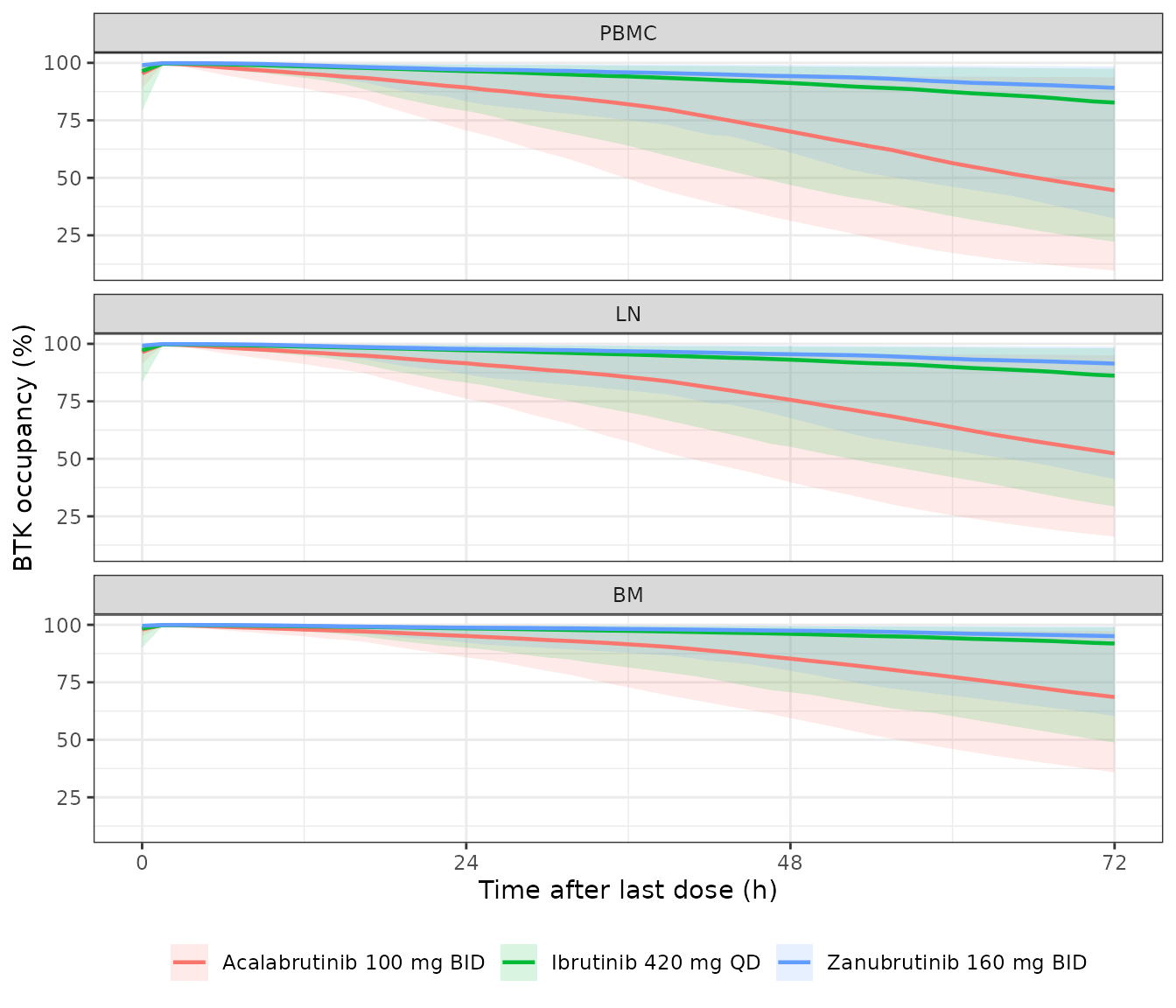
Median (band: 5th-95th percentile) BTK occupancy in the 72 h following the last dose. Replicates Figure 5 of Demin 2025.
Zanubrutinib holds the highest median occupancy in all three tissues across the interruption, ibrutinib is intermediate, and acalabrutinib falls fastest – reproducing the ordering and the approximate magnitudes in Figure 5 of the source, including acalabrutinib landing in the 60-70% range in PBMCs by 72 h.
Dose modification (Figure 6)
reduced <- tibble::tribble(
  ~arm,             ~cmt,      ~label,                    ~dose, ~ii,
  "Zanubrutinib",   "gut_zan", "160 mg BID (label)",      160,   0.5,
  "Zanubrutinib",   "gut_zan", "80 mg BID (reduction 1)",  80,   0.5,
  "Zanubrutinib",   "gut_zan", "80 mg QD (reduction 2)",   80,   1.0,
  "Acalabrutinib",  "gut_aca", "100 mg BID (label)",      100,   0.5,
  "Acalabrutinib",  "gut_aca", "100 mg QD (reduction 1)", 100,   1.0,
  "Ibrutinib",      "gut_ibr", "420 mg QD (label)",       420,   1.0,
  "Ibrutinib",      "gut_ibr", "280 mg QD (reduction 1)", 280,   1.0,
  "Ibrutinib",      "gut_ibr", "140 mg QD (reduction 2)", 140,   1.0
)

dose_mod <- lapply(seq_len(nrow(reduced)), function(i) {
  ev <-
    et(amt = reduced$dose[i], cmt = reduced$cmt[i],
       ii = reduced$ii[i], until = LAST_DOSE) %>%
    et(LAST_DOSE)
  s <- rxSolve(typical, ev, atol = 1e-9, rtol = 1e-7)
  s <- s[nrow(s), ]
  tibble::tibble(
    arm = reduced$arm[i], label = reduced$label[i],
    PBMC = s$occupancy_pbmc, LN = s$occupancy_ln, BM = s$occupancy_bm
  )
}) %>%
  dplyr::bind_rows()
#> ℹ omega/sigma items treated as zero: 'etald1_zan', 'etalvc_zan', 'etalvp_zan', 'etalcl_zan', 'etalq_zan', 'etalvc_aca', 'etalcl_aca', 'etalvc_acp', 'etalvp_acp', 'etalcl_acp', 'etalq_acp', 'etald1_ibr', 'etalvc_ibr', 'etalvp_ibr', 'etalcl_ibr', 'etalkabs_pci', 'etalclmet_ibr', 'etalcl_pci', 'etalatp', 'etalkdeg_btk', 'etaiovlvc_zan', 'etaiovlcl_zan', 'etaiovlmtt_aca', 'etaiovlf1_aca', 'etaiovlcl_ibr', 'etaiovlcl_pci'
#> ℹ omega/sigma items treated as zero: 'etald1_zan', 'etalvc_zan', 'etalvp_zan', 'etalcl_zan', 'etalq_zan', 'etalvc_aca', 'etalcl_aca', 'etalvc_acp', 'etalvp_acp', 'etalcl_acp', 'etalq_acp', 'etald1_ibr', 'etalvc_ibr', 'etalvp_ibr', 'etalcl_ibr', 'etalkabs_pci', 'etalclmet_ibr', 'etalcl_pci', 'etalatp', 'etalkdeg_btk', 'etaiovlvc_zan', 'etaiovlcl_zan', 'etaiovlmtt_aca', 'etaiovlf1_aca', 'etaiovlcl_ibr', 'etaiovlcl_pci'
#> ℹ omega/sigma items treated as zero: 'etald1_zan', 'etalvc_zan', 'etalvp_zan', 'etalcl_zan', 'etalq_zan', 'etalvc_aca', 'etalcl_aca', 'etalvc_acp', 'etalvp_acp', 'etalcl_acp', 'etalq_acp', 'etald1_ibr', 'etalvc_ibr', 'etalvp_ibr', 'etalcl_ibr', 'etalkabs_pci', 'etalclmet_ibr', 'etalcl_pci', 'etalatp', 'etalkdeg_btk', 'etaiovlvc_zan', 'etaiovlcl_zan', 'etaiovlmtt_aca', 'etaiovlf1_aca', 'etaiovlcl_ibr', 'etaiovlcl_pci'
#> ℹ omega/sigma items treated as zero: 'etald1_zan', 'etalvc_zan', 'etalvp_zan', 'etalcl_zan', 'etalq_zan', 'etalvc_aca', 'etalcl_aca', 'etalvc_acp', 'etalvp_acp', 'etalcl_acp', 'etalq_acp', 'etald1_ibr', 'etalvc_ibr', 'etalvp_ibr', 'etalcl_ibr', 'etalkabs_pci', 'etalclmet_ibr', 'etalcl_pci', 'etalatp', 'etalkdeg_btk', 'etaiovlvc_zan', 'etaiovlcl_zan', 'etaiovlmtt_aca', 'etaiovlf1_aca', 'etaiovlcl_ibr', 'etaiovlcl_pci'
#> ℹ omega/sigma items treated as zero: 'etald1_zan', 'etalvc_zan', 'etalvp_zan', 'etalcl_zan', 'etalq_zan', 'etalvc_aca', 'etalcl_aca', 'etalvc_acp', 'etalvp_acp', 'etalcl_acp', 'etalq_acp', 'etald1_ibr', 'etalvc_ibr', 'etalvp_ibr', 'etalcl_ibr', 'etalkabs_pci', 'etalclmet_ibr', 'etalcl_pci', 'etalatp', 'etalkdeg_btk', 'etaiovlvc_zan', 'etaiovlcl_zan', 'etaiovlmtt_aca', 'etaiovlf1_aca', 'etaiovlcl_ibr', 'etaiovlcl_pci'
#> ℹ omega/sigma items treated as zero: 'etald1_zan', 'etalvc_zan', 'etalvp_zan', 'etalcl_zan', 'etalq_zan', 'etalvc_aca', 'etalcl_aca', 'etalvc_acp', 'etalvp_acp', 'etalcl_acp', 'etalq_acp', 'etald1_ibr', 'etalvc_ibr', 'etalvp_ibr', 'etalcl_ibr', 'etalkabs_pci', 'etalclmet_ibr', 'etalcl_pci', 'etalatp', 'etalkdeg_btk', 'etaiovlvc_zan', 'etaiovlcl_zan', 'etaiovlmtt_aca', 'etaiovlf1_aca', 'etaiovlcl_ibr', 'etaiovlcl_pci'
#> ℹ omega/sigma items treated as zero: 'etald1_zan', 'etalvc_zan', 'etalvp_zan', 'etalcl_zan', 'etalq_zan', 'etalvc_aca', 'etalcl_aca', 'etalvc_acp', 'etalvp_acp', 'etalcl_acp', 'etalq_acp', 'etald1_ibr', 'etalvc_ibr', 'etalvp_ibr', 'etalcl_ibr', 'etalkabs_pci', 'etalclmet_ibr', 'etalcl_pci', 'etalatp', 'etalkdeg_btk', 'etaiovlvc_zan', 'etaiovlcl_zan', 'etaiovlmtt_aca', 'etaiovlf1_aca', 'etaiovlcl_ibr', 'etaiovlcl_pci'
#> ℹ omega/sigma items treated as zero: 'etald1_zan', 'etalvc_zan', 'etalvp_zan', 'etalcl_zan', 'etalq_zan', 'etalvc_aca', 'etalcl_aca', 'etalvc_acp', 'etalvp_acp', 'etalcl_acp', 'etalq_acp', 'etald1_ibr', 'etalvc_ibr', 'etalvp_ibr', 'etalcl_ibr', 'etalkabs_pci', 'etalclmet_ibr', 'etalcl_pci', 'etalatp', 'etalkdeg_btk', 'etaiovlvc_zan', 'etaiovlcl_zan', 'etaiovlmtt_aca', 'etaiovlf1_aca', 'etaiovlcl_ibr', 'etaiovlcl_pci'

dose_mod %>%
  tidyr::pivot_longer(c(PBMC, LN, BM), names_to = "tissue",
                      values_to = "occ") %>%
  dplyr::mutate(tissue = factor(tissue, levels = c("PBMC", "LN", "BM"))) %>%
  ggplot(aes(label, occ, fill = tissue)) +
  geom_col(position = "dodge") +
  coord_cartesian(ylim = c(80, 100)) +
  facet_wrap(~arm, scales = "free_x") +
  labs(x = NULL, y = "Trough BTK occupancy (%)", fill = NULL) +
  theme_bw() +
  theme(axis.text.x = element_text(angle = 30, hjust = 1),
        legend.position = "bottom")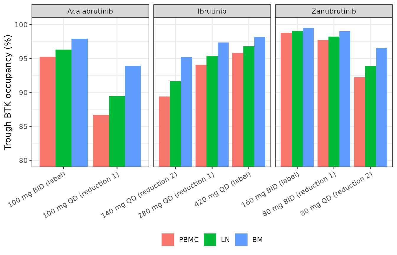
Typical-value trough BTK occupancy at the labelled dose and at the reduced doses recommended in each product label. Replicates Figure 6 of Demin 2025.
Consistent with Figure 6 of the source, the first dose reduction leaves zanubrutinib and ibrutinib at or above roughly 95% trough occupancy, whereas acalabrutinib drops below 90% in PBMCs and LNs.
Assumptions and deviations
The executable Heta model in the Supporting Information is treated as the authoritative specification, because it is the artefact that generated the published figures and tables. Where it disagrees with Table S1, the code wins and the disagreement is recorded here.
D1^zanis 0.0513 day, not the 0.513 printed in Table S1. The model code givesD1_zan_mean = 0.0513416day (1.23 h) and Table S1 prints0.513with the unit “Unitless”. The printed value is a factor-of-10 typo: the sibling entryD1^ibragrees exactly between the two sources (0.0412 day), and simulating both readings against the paper’s own Table 1 settles it. Using 0.0513 day gives 96.5 / 69.5 / 47.0 / 31.5% of patients above 95% occupancy in PBMCs at trough and 24 / 48 / 72 h, against the published 93.7 / 59.3 / 37.2 / 24.9%; using 0.513 day gives 100 / 99.0 / 78.5 / 53.5%, which is grossly inconsistent with the source’s own result. The model file uses 0.0513 day.Inter-occasion variability is encoded as a second subject-level random effect. In the Heta model each
iov_*term is aConst, i.e. a single value per virtual patient held constant for the whole simulation, rather than a deviate resampled at each dosing occasion. The IOV therefore behaves as an additional between-subject variance term in the artefact that produced the published results, and it is encoded that way here (etaiovl*), which reproduces the published spread. Users who want true occasion-level resampling must add an occasion column and index these etas by it.Vp^acacarries theVc^acarandom effect. The model code setsVd_prf_aca = Vp_aca_mean * exp(bsv_vc_aca)– the central-volume eta – while Table S1 reports a distinct 33.7% CV forVp^aca. This looks like a copy-paste slip in the source code, but it is what generated the published results, so it is reproduced here andVp^acahas no eta of its own.ALAG^ibris held constant. Table S1 reports 80.6% CV IIV on the ibrutinib absorption lag time, but the Heta model consumesalag_ibrinside its event scheduler and its own annotation states that the variability “cannot be implemented”. The constant is used here so the simulations match the published output. rxode2 would allow the IIV viaalag(); users who want it can add an eta toalag_ibr.No residual-error model. The source reports none: it is a deterministic mechanism model with a sampled virtual population, and predictions are compared as medians and 95% CI bands rather than fitted to individual observations. Nothing was invented to fill the gap.
Six convention warnings are expected.
checkModelConventions()reports thatetaiovlvc_zan,etaiovlcl_zan,etaiovlmtt_aca,etaiovlf1_aca,etaiovlcl_ibrandetaiovlcl_pcihave no matching fixed-effect parameter. That is inherent to the IOV naming idiom (the same warnings arise forBarnett_2018_coproporphyrin_I): the IOV eta shares its fixed effect with the corresponding IIV eta. No compartment or source-trace warnings remain.Cohort size. This vignette uses 200 virtual patients per arm against the source’s 1000, to keep the render inside the package’s time budget. All comparisons above are therefore reported with the binomial Monte Carlo standard error of a 200-subject cohort.
Residual disagreement. With those choices the reimplementation matches the published percentages closely at trough (all nine tissue-by-regimen comparisons within about 2 Monte Carlo SE) and through the interruption for ibrutinib (every one of its nine interruption cells within
|z| <= 2.0, and three of them within 0.3 percentage points). The zanubrutinib washout is the weakest point: simulated occupancy decays a little more slowly than published, leaving roughly 6-12 percentage points more patients above 95% at 24-72 h after the last dose. The trough values agree, the ordering of the three drugs is preserved at every timepoint and in every tissue, and the discrepancy is far smaller than the alternativeD1reading would produce, but it is not fully resolved from the available sources.Read the
zcolumn with care in the tail. Where the published percentage is close to zero – acalabrutinib at 48-72 h, published 0.8-5.7% – the binomial standard error is very small, so a difference of only 2-3 percentage points (e.g. simulated 5.0% versus published 1.6% in LN at 72 h) produceszvalues around 3-4. Those cells are a small absolute disagreement, not a large one;zis a useful yardstick in the middle of the range and a misleading one at the extremes.
Reference
Demin O Jr, Ou Y, Kolesova G, Shchelokov D, Stepanov A, Musatova V, Sahasranaman S, Zhao Y, Liu X, Tang Z, Hanley WD. Quantitative Systems Pharmacology Model to Predict Target Occupancy by Bruton Tyrosine Kinase Inhibitors in Patients With B-Cell Malignancies. CPT Pharmacometrics Syst Pharmacol. 2025;14(4):706-717. doi:10.1002/psp4.13307