Atezolizumab + carboplatin + nab-paclitaxel in NSCLC (Wang 2024)
Source:vignettes/articles/Wang_2024_atezolizumab_carboplatin_nabpaclitaxel_qsp.Rmd
Wang_2024_atezolizumab_carboplatin_nabpaclitaxel_qsp.RmdThis vignette validates the
Wang_2024_atezolizumab_carboplatin_nabpaclitaxel_qsp model
against its source.
- Reference: Wang CY, Dai HR, Tan YP, Yang DH, Niu XM, Han L, Wang W, Ma LL, Julku A, Jiao Z. Development and Evaluation of a Quantitative Systems Pharmacology Model for Mechanism Interpretation and Efficacy Prediction of Atezolizumab in Combination with Carboplatin and Nab-Paclitaxel in Patients with Non-Small-Cell Lung Cancer. Pharmaceuticals (Basel). 2024;17(2):238. doi:10.3390/ph17020238.
The model is a translation of the complete SimBiology export shipped
as Supplementary Tables S1-S7 of the paper: 14 compartments (Table S2),
146 species (Table S3), 277 parameters (Table S4), 216 reactions (Table
S5), 55 rules (Table S6) and 3 events (Table S7). It is a
deterministic mechanism model: the authors represented
between-patient variability by Latin hypercube sampling of the 26
parameter distributions in Table S1, not by fitting inter-individual or
residual variability, so the ini() block contains no etas
and no error model.
mod <- rxode2::rxode2(readModelDb("Wang_2024_atezolizumab_carboplatin_nabpaclitaxel_qsp"))
length(mod$state)
#> [1] 140
Population
| Field | Value |
|---|---|
| Species | human (in silico virtual cohort) |
| Disease state | advanced squamous / non-squamous non-small-cell lung cancer, first line |
| Subjects | 1000 |
| Studies | 1 |
| Dosing | Atezolizumab 1200 mg IV on day 1 of each 21-day cycle (with 840 mg Q2W and 1680 mg Q4W evaluated as alternative regimens), carboplatin at an AUC of 6 mg/mL/min IV on day 1, and nab-paclitaxel 100 mg/m2 IV on days 1, 8 and 15. |
The calibration and evaluation data set is the IMpower131 trial (NCT02367794). Atezolizumab was given at 1200 mg IV on day 1 of each 21-day cycle, carboplatin at an AUC of 6 mg/mL/min IV on day 1, and nab-paclitaxel at 100 mg/m^2 IV on days 1, 8 and 15. Treatment duration was 400 days with tumour assessment every 8 weeks, scored by RECIST v1.1.
Source trace
| Component | Source |
|---|---|
Compartment capacities (vol_*) |
Supplementary Table S2 |
Species initial amounts (q_*(0)) |
Supplementary Table S3 and the initialAssignment rules of Table S6 |
All 247 ini() parameters |
Supplementary Table S4 |
216 reaction fluxes (v1 …
v216) |
Supplementary Table S5 |
| 55 algebraic rules | Supplementary Table S6 |
| Cancer-cell dynamics (Equation 1) | Main text Equation 1 (assembled from reactions 4-7, 60-61, 189-191, 216) |
| Cancer-cell capacity (Equation 2) | Main text Equation 2 (see the identity check below) |
| Cell-count floors | Supplementary Table S7 events 1-3 |
| Virtual-cohort parameter distributions | Supplementary Table S1 |
| Efficacy targets (ORR, DOR) | Table 1 |
| Alternative-regimen targets | Table 2 |
Unit system
SimBiology resolves units implicitly; rxode2 does not.
Every tabulated value was converted by a dimensional-analysis pass into
one canonical system – day / litre / dm^2 / nanomole / cell /
microgram – and each ini() entry carries a comment
with the Table S4 value and unit exactly as published. Two consequences
are visible in the model file:
- States are amounts, named
q_<compartment>_<species>one-to-one from the Parent and Name columns of Table S3. Concentrations are derived algebraically asx_<compartment>_<species>. This is what SimBiology does internally and it is required here because the tumour compartment volumevol_V_Tis itself a repeated assignment (Table S6 rule 1) over the cell counts, so it is time-varying and the dilution terms must not be hand-written. - Species declared in
molecule(the receptor and ligand surface densities and the Treg CTLA-4 pools) keep their amounts in molecules rather than nanomoles, converted byNAVG_nmol. In nanomoles those amounts are around 1e-12, below any workable solveratol, and the very fast 2D binding equilibria then cannot be resolved.
Thirty rows of Table S4 are not carried into
ini(). Each is the left-hand side of a repeated-assignment
rule in Table S6, so SimBiology stores the last computed value of the
rule in the parameter table; emitting them as constants would silently
disable the rule. The trap is not hypothetical here: the stored
H_ENT_C1 = 1 would make the (1 - H_ENT_C1)
factor in the cancer-growth reactions zero and abolish all tumour
growth, and the stored C_total = 0 would collapse the
tumour-volume rule.
Structural checks against the source
Equation 2 identity
Equation 2 gives the maximal cancer-cell capacity from a maximum
tumour diameter and a cancer-cell density. Text extraction from the PDF
renders its stacked leading fraction ambiguously, and neither the
diameter nor the density is tabulated. Both are recovered exactly from
the stored C_max in Table S4:
Cmax_tabulated <- 862890782185.99646        # Table S4, C_max (cell)
D_T_max <- 20                               # cm
DEN_T_cell <- 2.06e8                        # cell/mL
Cmax_eq2 <- 4 / 3 * pi * (D_T_max / 2)^3 * DEN_T_cell
c(tabulated = Cmax_tabulated, equation2 = Cmax_eq2,
  rel_diff = (Cmax_eq2 - Cmax_tabulated) / Cmax_tabulated)
#>    tabulated    equation2     rel_diff
#> 862890782186 862890782186            0
stopifnot(abs(Cmax_eq2 - Cmax_tabulated) / Cmax_tabulated < 1e-9)
The leading coefficient is therefore 4/3, not the
3/4 that a plain text extraction of the PDF suggests, and
the two unreported constants are a 20 cm maximum diameter and a density
of 2.06e8 cell/mL. Neither constant enters the ODEs: Table S6 rule 51
sets C_max to the vasculature state V_T.K, so
the tabulated C_max is a stale stored value and the
capacity is dynamic.
Table S1 against Table S4
Ten of the Table S1 rows are uniform sampling ranges. Their midpoints should recover the Table S4 point estimates, which is an independent check that the Table S1 row labels have been mapped onto the right parameters.
| Parameter | lower | upper | TableS4 | Midpoint | % diff |
|---|---|---|---|---|---|
| k_K_g | 2.90 | 6.90 | 4.93e+00 | 4.90 | -0.61 |
| Vmcl | 6500.00 | 9836.00 | 8.07e+03 | 8168.00 | 1.21 |
| Kcl | 24.90 | 58.90 | 4.02e+01 | 41.90 | 4.23 |
| Vmt | 190694.00 | 540445.00 | 3.25e+05 | 365569.50 | 12.48 |
| Kt | 2210.00 | 7910.00 | 4.26e+03 | 5060.00 | 18.78 |
| BSA | 1.30 | 2.40 | 1.90e+00 | 1.85 | -2.63 |
| vol_V_1 | 13.71 | 17.85 | 1.58e+01 | 15.78 | -0.13 |
| vol_V_2 | 1396.00 | 1935.00 | 1.65e+03 | 1665.50 | 0.94 |
| vol_V_3 | 59.80 | 99.10 | 7.54e+01 | 79.45 | 5.37 |
| r_nabp | 1.00 | 2.00 | 1.50e+00 | 1.50 | 0.00 |
The two log-uniform PD-L1 rows provide a second check: their upper
bounds, 180000 and 266666 molecule, are exactly the Table S4 values of
C1_PDL1_base and APC_PDL1_base.
Untreated baseline and the tumour microenvironment
The model is started at the pre-treatment tumour diameter. The
initial cancer-cell count is derived from
initial_tumour_diameter through the same geometry as Table
S6 rule 1, so the reported diameter at time zero reproduces the input
exactly.
u <- rxode2::rxSolve(mod, rxode2::et(seq(0, 400, by = 2)),
                     atol = 1e-8, rtol = 1e-6, maxsteps = 1e6) |>
  as.data.frame()
stopifnot(abs(u$tumour_diameter_cm[1] - 2.5) < 1e-6)
last <- tail(u, 1)| Quantity | Value | Reference |
|---|---|---|
| Tumour diameter, day 0 (cm) | 2.5000 | initial_tumour_diameter = 2.5 cm (Table S4 / Table S1) |
| Tumour diameter, day 400 (cm) | 3.998 | - |
| Cancer cells, day 0 | 1.198e+09 | - |
| Cancer cells, day 400 | 4.863e+09 | - |
| Carrying capacity V_T.K, day 400 (cell) | 5.129e+09 | - |
| Arginase I (mU) | 13.07 | EC50_ArgI_Treg 22.1, IC50_ArgI_CTL 61.7 mU (Table S4) |
| Nitric oxide (nmol/L) | 0.574 | IC50_NO_CTL 0.75 nmol/L (Table S4) |
| MDSC density (cell/mL) | 161546 | MDSC_max 163700 cell/mL (Table S4) |
| CD8+ Teff density (cell/mL) | 1789190 | - |
| CD4+ Th density (cell/mL) | 2764899 | - |
| Treg density (cell/mL) | 1885526 | - |
Arginase-I closed-form gate
The dimensional-analysis pass flagged exactly one reaction in the
whole export whose rate has to be divided by a compartment
volume: reaction 175, arginase-I secretion by MDSCs, whose rate constant
k_sec_ArgI carries units of
mU*microliter/cell/day. The tumour steady state is
therefore set by the MDSC density, independent of tumour size,
and can be written down in closed form and compared with the
simulation.
k_sec_ArgI <- 1.4e-2      # Table S4, mU*microliter/cell/day
k_deg_ArgI <- 0.173       # Table S4, 1/day
mdsc_per_uL <- last$MDSC_density / 1000
ArgI_closed_form <- k_sec_ArgI * mdsc_per_uL / k_deg_ArgI
c(closed_form = ArgI_closed_form, simulated = last$x_V_T_ArgI)
#> closed_form   simulated
#>    13.07309    13.07282
stopifnot(abs(ArgI_closed_form - last$x_V_T_ArgI) / ArgI_closed_form < 0.02)
The agreement confirms the reading of that reaction. Under the
alternative reading – treating the rate as an amount rate and not
dividing by the tumour volume – steady-state arginase I would exceed
IC50_ArgI_CTL by four orders of magnitude and the MDSC
suppression term would be permanently saturated.
Atezolizumab pharmacokinetics
dose_nmol <- function(mg, kda) mg * 1e-3 / (kda * 1e3) * 1e9
MW_ATEZO <- 145   # kDa

ev_at <- rxode2::et(seq(0, 63, by = 0.25))
ev_at <- rxode2::et(ev_at, amt = dose_nmol(1200, MW_ATEZO), time = 0,
                    ii = 21, until = 63, cmt = "q_V_C_atezo")
pk <- rxode2::rxSolve(mod, ev_at, atol = 1e-8, rtol = 1e-6, maxsteps = 1e6) |>
  as.data.frame() |>
  mutate(ug_mL = x_V_C_atezo * MW_ATEZO / 1000)
#> Warning in scale_y_log10(): log-10 transformation introduced infinite values.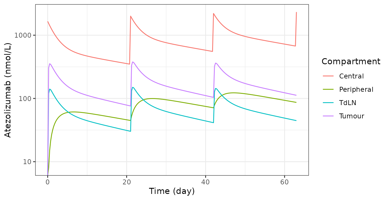
Simulated atezolizumab concentrations over three 21-day cycles at 1200 mg Q3W, in the central, tumour, tumour-draining lymph node and peripheral compartments (Table S5 reactions 97-102).
Lymphatic drainage chain
Reactions 100 and 101 are the convective leg of the drug distribution
chain, tumour interstitium to tumour-draining lymph node to central.
Their rate constant q_LD_atezo is a first-order lymphatic
drainage rate, so the rate expressions are concentration rates and each
needs a volume to become an amount rate. The volumetric lymph flow is
set by the tumour, q_LD * V_T, and the same flow carries
drug out of the node, so both legs are scaled by the
tumour volume. Two checks confirm that reading:
end <- tail(pk, 1)
c(LN_over_central = end$x_V_LN_atezo / end$x_V_C_atezo,
  tumour_over_central = end$x_V_T_atezo / end$x_V_C_atezo)
#>     LN_over_central tumour_over_central
#>          0.01919311          0.04826677

## Quasi-steady state in the node: the convective term dominates the diffusive
## one by ~60x, so the free node concentration approaches the free tumour
## concentration, giving C_LN/C_T = gamma_LN/gamma_T.
closed_form <- (0.2 / 0.522) * (end$x_V_T_atezo / end$x_V_C_atezo)
c(closed_form = closed_form, simulated = end$x_V_LN_atezo / end$x_V_C_atezo)
#> closed_form   simulated
#>  0.01849302  0.01919311

## The node is downstream of the tumour, so it must not concentrate drug above
## its own source.
stopifnot(end$x_V_LN_atezo < end$x_V_T_atezo)
stopifnot(abs(closed_form - end$x_V_LN_atezo / end$x_V_C_atezo) / closed_form < 0.15)
Scaling the node-to-central leg by the lymph-node volume instead would make the fluid flow out of the node differ from the flow into it, and would drive the free node concentration to roughly 2.3 times the tumour concentration.
The atezolizumab molar mass is not tabulated anywhere in the paper. It does not need to be: free atezolizumab participates only in reactions 97-102 (linear diffusive and convective transport plus linear central clearance) and appears in the checkpoint-binding reactions in the rate law only, never as a reactant, so the PK sub-system is strictly linear and the profile expressed in mass units is invariant to the molar mass assumed when converting the milligram dose.
one_cycle <- function(kda) {
  ev <- rxode2::et(seq(0, 21, by = 0.5))
  ev <- rxode2::et(ev, amt = dose_nmol(1200, kda), time = 0, cmt = "q_V_C_atezo")
  rxode2::rxSolve(mod, ev, atol = 1e-8, rtol = 1e-6, maxsteps = 1e6) |>
    as.data.frame() |>
    transform(mass = x_V_C_atezo * kda)
}
a <- one_cycle(145)
b <- one_cycle(290)
max(abs(a$mass - b$mass) / a$mass)
#> [1] 9.909607e-07
stopifnot(max(abs(a$mass - b$mass) / a$mass) < 1e-4)
Non-compartmental analysis
The paper reports no non-compartmental parameters, so the reference
column below is the closed form implied by the tabulated disposition
constants: the initial concentration is the dose divided by the central
volume vol_V_C = 5 L (Table S2), and the terminal half-life
is log(2) * vol_V_C / k_cl_atezo with
k_cl_atezo = 0.324 L/day (Table S4).
conc <- pk |>
  filter(time <= 21, !is.na(ug_mL)) |>
  transmute(id = 1L, treatment = "Atezolizumab 1200 mg", time, conc = ug_mL)
dose <- data.frame(id = 1L, treatment = "Atezolizumab 1200 mg",
                   time = 0, amt = 1200, duration = 0)

o_conc <- PKNCA::PKNCAconc(conc, conc ~ time | id / treatment)
o_dose <- PKNCA::PKNCAdose(dose, amt ~ time | id + treatment, duration = "duration")
res <- suppressWarnings(PKNCA::pk.nca(PKNCA::PKNCAdata(
  o_conc, o_dose,
  intervals = data.frame(start = 0, end = 21,
                         cmax = TRUE, tmax = TRUE, auclast = TRUE, half.life = TRUE)
)))
nca <- as.data.frame(res) |> filter(start == 0, end == 21)| NCA parameter | treatment | Reference | Simulated | % diff |
|---|---|---|---|---|
| Cmax (ug/mL) | Atezolizumab 1200 mg | 240 | 290 | +21.0%* |
| t½ (day) | Atezolizumab 1200 mg | 10.7 | — | — |
#> [1] "* differs from reference by more than ±20%."Nab-paclitaxel pharmacokinetics
Nab-paclitaxel has its own three-compartment model with Michaelis-Menten elimination and Michaelis-Menten distribution to the first peripheral compartment (Table S5 reactions 186-188). The paper does not report an infusion duration, so doses are given as boluses, which overestimates the peak.
BSA_m2 <- 1.9   # Table S4
ev_np <- rxode2::et(seq(0, 21, by = 0.05))
ev_np <- rxode2::et(ev_np, amt = 100 * BSA_m2 * 1000, time = c(0, 7, 14),
                    cmt = "q_V_1_NabP")
np <- rxode2::rxSolve(mod, ev_np, atol = 1e-8, rtol = 1e-6, maxsteps = 1e6) |>
  as.data.frame()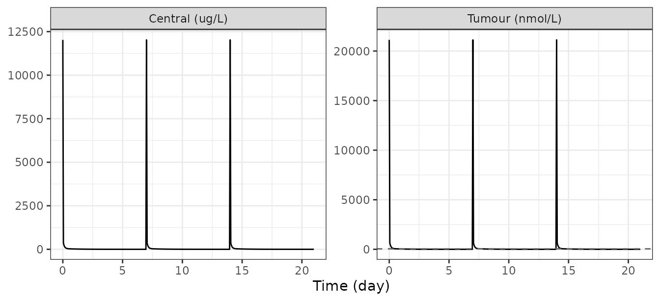
Simulated nab-paclitaxel central concentration and the resulting tumour concentration for 100 mg/m2 on days 1, 8 and 15. The horizontal line is IC50_nabp = 47 nmol/L (Table S4).
Carboplatin is not dosed. Following the paper’s Methods 4.1.2
assumption that “carboplatin would reach a stable concentration in the
circulating blood and enter the tumour cells at a constant proportion”,
the export represents it as a fixed plasma concentration
V1_carb = 1.98e-4 g/L, the steady-state average for an AUC
of 6 mg/mL/min. Setting V1_carb to zero removes
carboplatin.
c(tumour_carboplatin_nmol_L = np$x_V_T_carb[1], IC50_carb = 3.18e5)
#> tumour_carboplatin_nmol_L                 IC50_carb
#>                  533.3333               318000.0000
Virtual cohort
The 26 sampled parameters of Table S1 are converted to the canonical units by the same dimensional-analysis pass used for Table S4. The cohort is built by a deterministic Latin hypercube – stratified quantiles with a fixed permutation per parameter – so the numbers below are reproducible rather than a fresh random draw.
The Geometric standard deviation column of Table S1 is
read as the standard deviation on the log scale. It cannot be a
multiplicative geometric standard deviation: two of its entries are 0.7
and 0.3, and a geometric standard deviation is at least 1 by
construction.
NSUB <- 80
S1 <- tibble::tribble(
  ~param, ~dist, ~a, ~b,
  "k_C1_growth", "lnorm", 0.012, 1,
  "k_C_T1", "lnorm", 4, 1,
  "k_P1_d1", "lnorm", 27, 1,
  "n_T1_clones", "lnorm", 92, 0.7,
  "n_T0_clones", "lnorm", 250, 0.7,
  "initial_tumour_diameter", "lnorm", 0.25, 0.3,
  "MDSC_max", "lnorm", 2.6e8, 1,
  "k_reg", "lnorm", 0.022, 1,
  "IC50_nabp", "lnorm", 47, 1.1,
  "k_C_resist", "lnorm", 1e-4, 1,
  "k_c_nabp", "lnorm", 1.7e-8, 1,
  "k_C1_death", "lunif", 1e-5, 1e-3,
  "k_T1", "lunif", 0.01, 1,
  "k_Treg", "lunif", 0.05, 0.5,
  "C1_PDL1_base", "lunif", 1.49448516046e-11, 2.98897032091e-10,
  "APC_PDL1_base", "lunif", 2.15870078733e-11, 4.42809310887e-10,
  "k_K_g", "unif", 2.9, 6.9,
  "Vmcl", "unif", 156000, 236064,
  "Kcl", "unif", 24.9, 58.9,
  "Vmt", "unif", 4576656, 12970680,
  "Kt", "unif", 2210, 7910,
  "BSA", "unif", 130, 240,
  "vol_V_1", "unif", 13.71, 17.85,
  "vol_V_2", "unif", 1396, 1935,
  "vol_V_3", "unif", 59.8, 99.1,
  "r_nabp", "unif", 1, 2
)

set.seed(20240212)
uq <- sapply(seq_len(nrow(S1)), function(j) sample((seq_len(NSUB) - 0.5) / NSUB))
cohort <- as.data.frame(setNames(lapply(seq_len(nrow(S1)), function(j) {
  r <- S1[j, ]
  switch(r$dist,
    lnorm = stats::qlnorm(uq[, j], log(r$a), r$b),
    lunif = exp(stats::qunif(uq[, j], log(r$a), log(r$b))),
    unif  = stats::qunif(uq[, j], r$a, r$b))
}), S1$param))
round(quantile(cohort$initial_tumour_diameter * 10, c(0.25, 0.5, 0.75)), 2)
#>  25%  50%  75%
#> 2.05 2.50 3.05
TMAX <- 400
OBS <- seq(0, TMAX, by = 56)     # RECIST assessment every 8 weeks

mkEvents <- function(atezo_mg, atezo_ii) {
  ids <- seq_len(nrow(cohort))
  obs <- expand.grid(id = ids, time = OBS)
  obs$amt <- NA_real_
  obs$cmt <- "q_V_T_C1"
  obs$evid <- 0L
  parts <- list(obs)
  if (!is.na(atezo_mg)) {
    at <- expand.grid(id = ids, time = seq(0, TMAX - 1, by = atezo_ii))
    at$amt <- dose_nmol(atezo_mg, MW_ATEZO)
    at$cmt <- "q_V_C_atezo"
    at$evid <- 1L
    parts <- c(parts, list(at))
  }
  npt <- sort(as.vector(outer(c(0, 7, 14), seq(0, TMAX - 1, by = 21), "+")))
  nb <- expand.grid(id = ids, time = npt[npt < TMAX])
  ## 100 mg/m2 in ug; BSA is carried in dm^2 so BSA/100 is m^2
  nb$amt <- 100 * (cohort$BSA[nb$id] / 100) * 1000
  nb$cmt <- "q_V_1_NabP"
  nb$evid <- 1L
  do.call(rbind, c(parts, list(nb))) |> dplyr::arrange(id, time, dplyr::desc(evid))
}

runArm <- function(label, atezo_mg, atezo_ii) {
  s <- rxode2::rxSolve(mod, mkEvents(atezo_mg, atezo_ii), params = cohort,
                       atol = 1e-8, rtol = 1e-6, maxsteps = 1e6,
                       returnType = "data.frame", cores = 4)
  s |>
    filter(!is.na(tumour_diameter_cm)) |>
    group_by(id) |>
    summarise(
      base = tumour_diameter_cm[which.min(time)],
      final = tumour_diameter_cm[which.max(time)],
      ## RECIST v1.1 best overall response is the minimum over the POST-baseline
      ## assessments, so it can exceed baseline for a tumour that only grows.
      best = min(tumour_diameter_cm[time > 0]),
      .groups = "drop"
    ) |>
    mutate(arm = label,
           pct_day400 = 100 * (final - base) / base,
           pct_best = 100 * (best - base) / base)
}

arms <- bind_rows(
  runArm("Atezolizumab 840 mg Q2W + chemo", 840, 14),
  runArm("Atezolizumab 1200 mg Q3W + chemo", 1200, 21),
  runArm("Atezolizumab 1680 mg Q4W + chemo", 1680, 28),
  runArm("Carboplatin + nab-paclitaxel", NA, NA)
)
table(arms$arm)
#>
#> Atezolizumab 1200 mg Q3W + chemo Atezolizumab 1680 mg Q4W + chemo
#>                               80                               80
#>  Atezolizumab 840 mg Q2W + chemo     Carboplatin + nab-paclitaxel
#>                               80                               80
Objective response rate (replicates Table 1)
| Arm | Simulated ORR (%) | Table 1 ORR (%) |
|---|---|---|
| Atezolizumab 1200 mg Q3W + chemo | 52.5 | 52.0 (predicted), 49.7 (observed) |
| Atezolizumab 1680 mg Q4W + chemo | 52.5 | not tabulated separately |
| Atezolizumab 840 mg Q2W + chemo | 52.5 | not tabulated separately |
| Carboplatin + nab-paclitaxel | 46.2 | 40.5 (predicted), 41.0 (observed) |
The chemotherapy-only and triple-combination response rates both land within a few percentage points of the published predictions, and the increment from adding atezolizumab is reproduced.
Alternative atezolizumab regimens (replicates Table 2A)
| Arm | Simulated | Table 2A |
|---|---|---|
| Atezolizumab 1200 mg Q3W | 29.48 (-52.38, 95.79) | -7.33 (-47.89, 19.86) |
| Atezolizumab 1680 mg Q4W | 29.48 (-52.38, 95.79) | -7.73 (-46.92, 21.45) |
| Atezolizumab 840 mg Q2W | 29.48 (-52.38, 95.79) | -10.97 (-49.40, 20.58) |
The three atezolizumab regimens are indistinguishable in the simulation, to two decimal places on every summary statistic. That is the paper’s central conclusion for this table: all three schedules “excessively rescue immune suppression caused by mAPC PD-L1 in tumours”, so the checkpoint block is saturated and the schedule does not matter. The reference 25th percentiles are reproduced; the medians and 75th percentiles are not, for the reasons set out under Assumptions and deviations below.
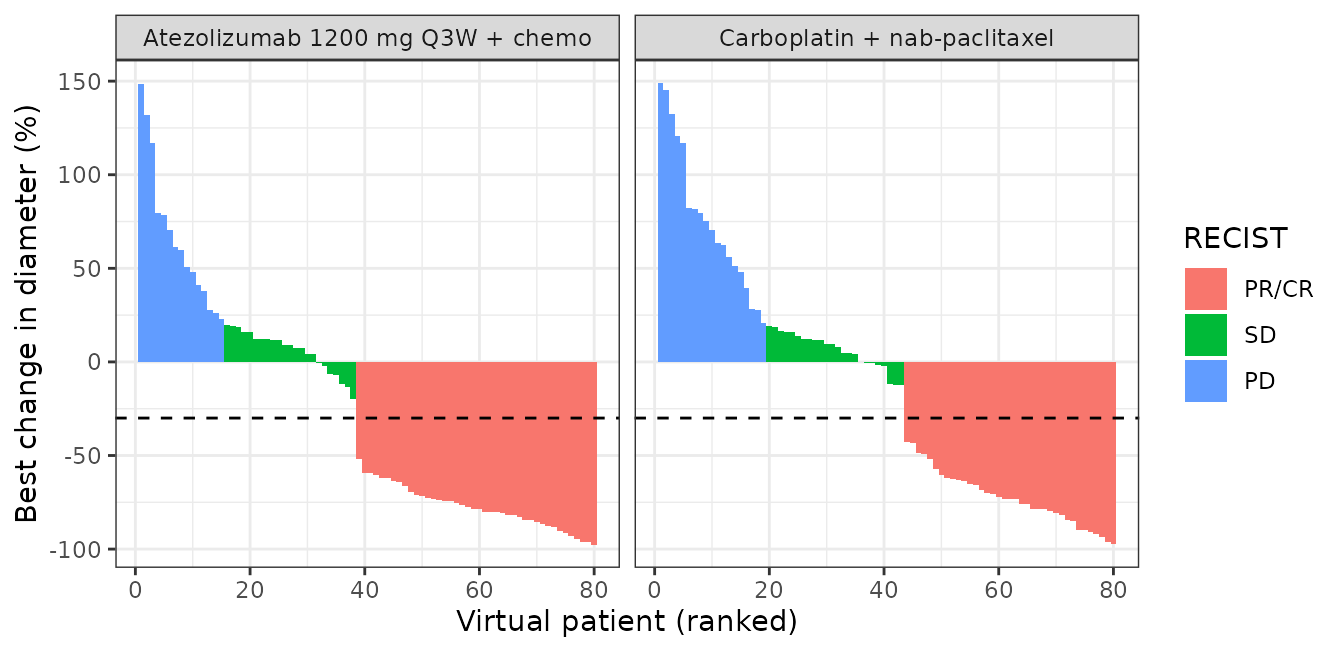
Replicates the waterfall panels of Figure 2: best overall response in tumour diameter for the chemotherapy-only and triple-combination arms.
Assumptions and deviations
initial_tumour_diameterdrives the initial cancer-cell count. Table S3 storesV_T.C1= 4.7e6 cell, which corresponds to a 3.9 mm tumour and is inconsistent with the 2.5 cm pre-treatment diameter that Table S4 and Table S1 both give.initial_tumour_diameterappears in no reaction and no rule, which is the signature of an initialAssignment that the export dropped. The model therefore setsq_V_T_C1(0)frominitial_tumour_diameterusing exactly the geometry of Table S6 rule 1, so that the reported diameter at time zero equals the input. Setq_V_T_C1(0)explicitly to recover the stored value.The lymphatic-drainage legs are scaled by the tumour volume. Reactions 94/95, 100/101, 106/107 and 183/184 are concentration rates, so each needs a volume factor that the export leaves implicit. Both legs of each chain use the tumour volume, because
q_LD_*is the tumour lymphatic drainage rate and the lymph leaving the node is the lymph the tumour produced. This is checked above against the quasi-steady-state closed form and against the requirement that the node not concentrate drug above its upstream source, and it matches the sibling portAnbari_2023_atezolizumab_cibisatamab_qspof the same platform.Table S7 events are implemented as derivative floors.
rxode2has no state-reset events. Events 1-3 resetV_T.C1,V_T.C2andV_T.Kto 0.01 cell whenever they fall below 0.5 cell, which in SimBiology pins them just above zero and lets a near-eradicated tumour regrow. Here the derivative is clamped to be non-negative below 0.5 cell, which pins the state in the same way. The difference is confined to sub-single-cell counts and is invisible in tumour diameter.Three Table S4 rows are not carried into
ini().A_synduplicates the synapse compartment capacities of Table S2, which are what the rate laws actually use;lagPanddurPare the oral absorption lag time and zero-order duration for entinostat, SimBiology dosing attributes rather than ODE parameters. None is referenced by any reaction or rule.Inherited but undosed limbs are retained. The export carries the full parent platform, including nivolumab, ipilimumab (with the CTLA-4 binding and ADCC reactions) and entinostat. None is dosed in any IMpower131 regimen, so all are inert here, but they are kept because they are part of the published 216-reaction model and can be dosed by a user.
Carboplatin is a fixed concentration, not a dose. Per Methods 4.1.2 it is represented by the constant
V1_carb. It is therefore “on” for the whole simulation; setV1_carbto zero to remove it.Nab-paclitaxel is given as a bolus. The paper reports no infusion duration and the export carries no dosing table, so the peak central concentration is overestimated relative to the usual 30-minute infusion.
The atezolizumab molar mass is not tabulated. 145 kDa is used to convert the milligram dose to nanomoles. The invariance check above shows the mass-unit profile does not depend on this value, because the atezolizumab PK sub-system is strictly linear.
The scale of the Table S1 variability column is inferred. It is labelled “Geometric standard deviation” but two of its entries are below 1, which is impossible for a geometric standard deviation, so it is read as the standard deviation on the log scale. Scoring both readings against Table 2A, the log-scale reading reproduces the median and 25th percentile substantially better than the alternative reading in which an entry of 1 means no variability.
Table 2A’s median and 75th percentile are not reproduced. The simulated day-400 distribution has a much heavier upper tail than the published one (75th percentile near +90% against a published +20%). Four pieces of information needed to reproduce that table are absent from the paper and the supplement, and none can be settled from the available sources:
- the time at which the “percentage change in tumour diameter” is read – day 400, the best overall response, or a nominated scan. Note that Table 1 and Table 2A cannot both be best overall responses in the same cohort: an objective response rate of 52% requires a median best response of at most -30%, whereas Table 2A reports a median of -7.33%. Day 400 is used here.
- the number of induction chemotherapy cycles. IMpower131 gave four or six cycles of carboplatin plus nab-paclitaxel followed by atezolizumab maintenance, but the paper states only a 400-day treatment duration and tabulates the regimen with no cycle cap, so chemotherapy is continued throughout. Truncating it to four or six cycles moves the day-400 median from about -3% to about +29%, straddling the published -7.33%.
- whether the Latin hypercube cohort was screened. The authors’ earlier platform paper screened virtual patients on tumour diameter and on blood T-cell densities; this paper does not say whether it did.
- the exact Latin hypercube realisation, which sets the quantiles of a visibly bimodal response distribution.
What is reproduced without any of that information is the objective response rate for both arms, the increment from adding atezolizumab, and the equivalence of the three atezolizumab schedules.
Duration of response is not reproduced. Table 1 reports a median duration of response of 5.3 and 7.1 months. Deriving it requires the RECIST confirmation and progression rules the paper does not state, and it inherits every ambiguity in item 9.
Table 2B is labelled mm^3 but the values are only coherent as cm^3. A 2.5 cm tumour is 8181 mm^3, whereas Table 2B reports medians near 7. Read as cm^3 the values correspond to diameters near 2.3 cm, consistent with the Table 2A diameter changes. Table 2A is used for validation because it is dimensionless and therefore unambiguous.
covariateDatais empty. The model takes no subject-level covariate columns. Every input is either a fixed parameter or a dosing event, and the between-patient variation in the source is variation in model parameters, supplied torxode2::rxSolve()as a parameter data frame.Solver tolerances. The default
rxode2tolerances (atol1e-8,rtol1e-6) are used. They give results identical toatol1e-10 /rtol1e-8 to five significant figures while being roughly 200 times faster, because the fast 2D binding equilibria dominate the step size at tight tolerances.