Model and source
- Citation: Cao Y, Willis BA, Horie K, Wildsmith KR, Koyama A, Sachdev P, Penner N, Charil A, Irizarry M, Reyderman L. Neuro-Dynamic Quantitative Systems Pharmacology (QSP) model describing Alzheimer’s disease pathophysiology and treatment effects. NPJ Syst Biol Appl. 2026;12(1):55. doi:10.1038/s41540-026-00677-4.
- Description: QSP. Neuro-Dynamic quantitative systems pharmacology model of Alzheimer’s disease pathophysiology and anti-amyloid treatment effects, with lecanemab as the reference drug. Eleven ODEs across three interlinked modules. Amyloid module: a four-stage reversible A-beta aggregation cascade (monomer A -> oligomer O -> protofibril F -> plaque P) in which F and P cooperatively accelerate every forward aggregation step. Tau module: five neuron states (N healthy, I0 minimal misfolded tau, I1 misfolded tau oligomers, I2 tau tangles, DN irreversible neurodegeneration) driven by spontaneous misfolding, tau-seed (TS) infection of healthy neurons, and amyloid promotion, plus a phosphorylated-tau pool (TP); transitions are reversible except into DN. Cognitive module: CDR-SB and ADAS-Cog are power functions of a weighted composite of I1, I2 and DN neuron fractions plus a direct amyloid-plaque effect. Six observables are fitted (amyloid PET Centiloid, medial-temporal tau PET SUVR, plasma A-beta 42/40 ratio, plasma p-tau181, CDR-SB, ADAS-Cog) and two are predicted but not fitted (CSF A-beta 42, CSF p-tau181). Lecanemab acts as additive first-order clearance on protofibrils and plaques, driven by the steady-state average serum concentration covariate CSS_LEC; the estimated protofibril effect is about 2.3-fold the plaque effect at the cohort median age. Model time is YEARS SINCE AD PATHOLOGICAL ONSET (not study time): the analysis dataset was aligned to a subject-specific onset using the GRACE method. Fitted by SAEM in Monolix 2021R1 to 4056 subjects from lecanemab Study 201, Study 301 (Clarity AD) Core and OLE, and the ADNI natural-history cohort. Of 74 parameters, 35 are fixed, 32 are estimated with IIV and 7 with fixed effects only.
- Article: https://doi.org/10.1038/s41540-026-00677-4
- Supplement (Supplementary Notes 1-7, Tables S1-S15, Figures S1-S22): https://static-content.springer.com/esm/art%3A10.1038%2Fs41540-026-00677-4/MediaObjects/41540_2026_677_MOESM1_ESM.pdf
The Neuro-Dynamic QSP model is a mechanistic description of the Alzheimer’s disease (AD) continuum. Eleven ODEs span three interlinked modules – an amyloid-beta aggregation cascade, a five-stage tau-pathology neuron chain, and a cognitive-decline module – and six clinical endpoints are fitted simultaneously. Lecanemab enters as additive clearance on the two aggregated amyloid species it binds.
Two things about this model are unusual and drive everything below.
Model time is years since AD pathological onset, not study
time. The analysis dataset was aligned to a subject-specific
onset estimated with the GRACE method, shifted by +20 years so all times
are positive. At t = 0 the model represents a person whose
amyloid-monomer production has begun but who has no aggregated amyloid,
no tau pathology, a negative amyloid PET, a negative tau PET and normal
cognition. Study 301 subjects enter the trial roughly 25-30 pathological
years later.
There are no dosing events. Drug exposure enters
through the time-varying covariate CSS_LEC, the
steady-state average serum concentration of lecanemab in ug/mL,
generated externally by the lecanemab population PK model. Setting
CSS_LEC = 0 turns the drug off; that is algebraically
identical to the paper’s
if (treatment window) ... else Eff = 1 construction and
generalises to any number of treatment and washout windows.
Because the model has no dosing, no PK compartment and no concentration-time profile, PKNCA is not an appropriate validation tool. This vignette follows the endogenous / mechanistic validation route instead: a mass-balance identity, an initial-condition check, reproduction of the published biomarker cascade, and comparison against the paper’s own quantitative claims and the Clarity AD (Study 301) published outcomes.
Population
pop <- attr(readModelDb("Cao_2026_lecanemab"), "population")The model was fitted to subjects across studies: lecanemab Study 201 (N = 854), Study 301 / Clarity AD (N = 1795) and the ADNI natural-history cohort (N = 1407). Baseline demographics come from Supplementary Table A1.
| Characteristic | ADNI | Study 201 | Study 301 |
|---|---|---|---|
| Age, mean (SD) years | 73.4 (7.7) | 71.3 (8.2) | 71.3 (7.8) |
| Baseline CDR-SB, mean (SD) | 2.3 (1.8) | 2.9 (1.4) | 3.2 (1.3) |
| Female | 41.7% | 49.4% | 52.2% |
| White | 92.9% | 90.6% | 76.9% |
| Asian (all categories) | 1.8% | 6.5% | 16.9% |
| APOE-e4 non-carrier / het / hom | 45.5 / 41.2 / 13.4% | 28.6 / 54.9 / 16.5% | 31.4 / 53.3 / 15.3% |
| Baseline diagnosis | EMCI 27.0%, LMCI 45.3%, mild AD dementia 27.6% | MCI 64.1%, mild dementia due to AD 35.9% | MCI 61.9%, mild dementia due to AD 38.1% |
ADNI subjects whose baseline diagnosis was cognitively normal or significant memory concern were excluded. ADNI plasma biomarkers and tau PET were excluded for assay incomparability, so tau PET comes only from a Study 301 substudy (N = 355).
Source trace
Every ini() value and every model()
equation, with its source location. The supplement is the primary source
for parameter values; the main article carries the ODE system and the
covariate narrative.
Equations
| Model component | Source location |
|---|---|
Amyloid ODEs (A, O, F,
P) |
Main text Eq 1; Methods “Full ODE system” > “Equations” |
Tau ODEs (N, I0, I1,
I2, DN, TS, TP) |
Main text Eq 2; Methods “Full ODE system” |
Cognitive equations (compEffCdr,
compEffAdas, CDRSB, ADASCOG) |
Main text Eq 3; Methods “Algebraic equation to derive clinical outcomes” |
Amyloid PET (ABSUVR, CENTILOID) |
Methods “Full ODE system”:
ABSUVR = sP * (fPFP * F + P) + ABSUVR0;
CENTILOID = ABSUVR * 236.6 - 246.9
|
Tau PET (TAUSUVR) |
Methods “Full ODE system”:
TAUSUVR = (sI2TAUPET * (fI1T * I1 + I2))^ShapeTau + TAUSUVR0
|
Fluid biomarkers (CSFAB, PAB,
CSFPTAU, PPTAU) |
Methods “Full ODE system” |
Drug effect (effLecaF, effLecaP) |
Methods “Full ODE system” > “Set up the drug effect of lecanemab on amyloid protofibrils and plaques” |
Initial conditions A(0), N(0)
|
Methods “Base model development stages” (only A and N non-zero at onset); values from Supplementary Note 2 |
Cap CDRSB <= 18, ADASCOG <= 90
|
Main text Eq 3 (“CDR-SB scores are capped at 18”; “ADAS-Cog total score is capped at 90”) |
Parameters
| Group | Count | Source table |
|---|---|---|
| Amyloid pathway | 19 | Supplementary Table S3 (final), S2 (fixed), Note 2 (derivations) |
| Tau pathway | 32 | Supplementary Table S6 (final), S5 (fixed), Note 3 (derivations) |
| Cognitive function | 15 | Supplementary Table S9 (final), S8 (fixed), Note 4; N0
from Note 2 |
| Protofibril / plaque contribution factors | 5 | Supplementary Table S12 (final), S11 (fixed) |
| Drug effect | 2 | Supplementary Table S13 |
| Covariate coefficients | 17 | Supplementary Table S14 |
| Residual error | 9 | Supplementary Table S14, “Final QSP Error Model Parameters” |
| Inter-individual variability | 32 | “Std dev of the random effects” columns of Tables S3, S6, S9, S13; correlations from Table S14 |
The per-parameter source location is carried as a trailing comment on
every ini() line of
inst/modeldb/specificDrugs/Cao_2026_lecanemab.R.
Parameter accounting reproduces the paper’s own count
The paper states: “The final QSP model contains 74 parameters, of which 35 were fixed, 32 were estimated with inter-subject variability, and 7 were estimated with only fixed effects.” The packaged model reproduces that split exactly, which is a complete-transcription check – a missed or invented parameter would break one of the three counts.
ui <- rxode2::rxode(readModelDb("Cao_2026_lecanemab"))
#> ℹ parameter labels from comments will be replaced by 'label()'

# Structural parameters only: exclude covariate coefficients (e_*) and
# residual-error terms (addSd_* / propSd_*), which the paper counts separately.
iniDf <- ui$iniDf
struct <- iniDf[!is.na(iniDf$ntheta) &
                  !grepl("^(e_|addSd_|propSd_)", iniDf$name), ]

etaNames <- iniDf$name[is.na(iniDf$ntheta)]
# etalpNA -> lpNA, so the IIV can be matched back to its theta.
etaTheta <- sub("^eta", "", etaNames)

nWithIIV     <- sum(struct$name %in% etaTheta)
nFixedNoIIV  <- sum(struct$fix & !(struct$name %in% etaTheta))
nEstNoIIV    <- sum(!struct$fix & !(struct$name %in% etaTheta))

accounting <- data.frame(
  Quantity = c("Total structural parameters",
               "Fixed (no IIV)",
               "Estimated with IIV",
               "Estimated, fixed effects only"),
  Model = c(nrow(struct), nFixedNoIIV, nWithIIV, nEstNoIIV),
  Paper = c(74L, 35L, 32L, 7L)
)
knitr::kable(accounting)| Quantity | Model | Paper |
|---|---|---|
| Total structural parameters | 74 | 74 |
| Fixed (no IIV) | 35 | 35 |
| Estimated with IIV | 32 | 32 |
| Estimated, fixed effects only | 7 | 7 |
Note that kDeAggPF and sF have a
fixed fixed-effect but an estimated IIV (Supplementary
Tables S3), so the paper counts them in the 32-with-IIV group rather
than the 35 fixed; the accounting above follows that convention.
Simulation set-up
mod  <- rxode2::rxode(readModelDb("Cao_2026_lecanemab"))
#> ℹ parameter labels from comments will be replaced by 'label()'
modT <- rxode2::zeroRe(mod)   # typical-value (all etas zero) version

# Cohort mean age in Studies 201 and 301 (Supplementary Table A1).
AGE_REF <- 71.3

# Reference-category subject: APOE-e4 non-carrier, baseline EMCI (all four
# DIS_AD_* stage indicators 0), non-Asian. This is the covariate combination
# the population estimates in Tables S3 / S6 / S9 / S13 refer to.
covRef <- list(
  AGE = AGE_REF, APOE4_HET = 0, APOE4_HOM = 0, APOE4_CARRIER = 0,
  RACE_ASIAN = 0, DIS_AD_LMCI = 0, DIS_AD_MCI = 0,
  DIS_AD_MILD = 0, DIS_AD_DEMENTIA = 0
)

# Lecanemab Css,av for the approved 10 mg/kg IV Q2W regimen. The value is
# reported only as a distribution in Supplementary Figure E21 (log-normal,
# mode near 115-130 ug/mL, median near 135 ug/mL, range about 30-370); 135 is
# a digitised median. See "Assumptions and deviations".
CSS_LEC_Q2W <- 135

#' Build an observation-only event table.
#'
#' The model declares six endpoints, so rxode2 requires every observation row
#' to name one; `dvid = 1L` with `cmt = NA_character_` is the form that works
#' regardless of how the endpoint slot indices line up against the 11 ODE
#' states. All observables are returned as columns on every row.
adEvents <- function(times, cssLec = 0, covs = covRef) {
  ev <- data.frame(id = 1L, time = times, evid = 0L,
                   cmt = NA_character_, dvid = 1L)
  ev$CSS_LEC <- cssLec
  for (nm in names(covs)) ev[[nm]] <- covs[[nm]]
  ev
}

#' Solve the typical-value model over a treatment window.
#'
#' @param txStart,txStop pathological times (years) bounding lecanemab dosing;
#'   `CSS_LEC` is `css` inside the window and 0 outside it.
#' Every solve must START AT TIME 0. The model's initial conditions (`A(0)`,
#' `N(0)`) are the disease-onset state, and rxode2 begins integrating at the
#' first record, so a solve whose first record is at trial entry would restart
#' the disease there instead of inheriting 27 years of accumulated pathology.
#'
#' `covsInterpolation = "locf"` makes `CSS_LEC` a true step function. The
#' default (linear) would ramp the concentration between records rather than
#' switching it, which is not what the paper's if/else construction means.
adSolve <- function(txStart = Inf, txStop = Inf, css = CSS_LEC_Q2W,
                    tmax = 45, by = 1 / 12, covs = covRef, model = modT) {
  ev <- adEvents(seq(0, tmax, by = by), covs = covs)
  ev$CSS_LEC <- ifelse(ev$time >= txStart & ev$time < txStop, css, 0)
  as.data.frame(rxode2::rxSolve(model, ev, atol = 1e-10, rtol = 1e-10,
                                method = "lsoda", covsInterpolation = "locf",
                                returnType = "data.frame"))
}

#' Nearest solved record to a requested time.
atTime <- function(d, tt) d[which.min(abs(d$time - tt)), , drop = FALSE]

natural <- adSolve()   # no treatment, 45 pathological years
#> ℹ omega/sigma items treated as zero: 'etalkAggAO', 'etalalphaCdr', 'etalpNA', 'etalDELECAP', 'etalDELECAF', 'etalehcAdas', 'etalshapeAdas', 'etalalphaAdas', 'etalehcCdr', 'etalshapeCdr', 'etalsI2TAUPET', 'etalTAUSUVR0', 'etalPPTAUFLOOR', 'etalpPI1', 'etalpPI0', 'etalpSI1', 'etalpSI0', 'etaltI12', 'etaltI01', 'etalsTauP', 'etalsTauS', 'etalPABFLOOR', 'etalABSUVR0', 'etalcP', 'etalcF', 'etalsP', 'etalsF', 'etalsO', 'etalsA', 'etalkDeAggPF', 'etalkAggFP', 'etalkDeAggOA'
Structural check 1: neuron mass balance
The five neuron states form a closed compartmental system. Every
transition appears once as an efflux and once as an influx, and
DN is a pure sink, so N + I0 + I1 + I2 + DN
must equal N0 for all time. This is an exact algebraic
identity of the transcribed ODEs, not a statistical comparison, so a
tight tolerance is the correct assertion: a sign error, a dropped
recovery term or a mismatched flux between any two neuron states breaks
it immediately.
N0 <- 6.14e7   # Supplementary Note 2: 86e9 neurons / 1400 mL brain volume
neuronTotal <- with(natural, N + I0 + I1 + I2 + DN)
relErr <- abs(neuronTotal - N0) / N0

cat(sprintf("max |relative deviation from N0| over %.0f years: %.3g\n",
            max(natural$time), max(relErr)))
#> max |relative deviation from N0| over 45 years: 3.51e-14

stopifnot(max(relErr) < 1e-6)
Structural check 2: the disease-onset initial condition
The paper defines t = 0 as a state in which
amyloid-monomer production has started but nothing has aggregated, tau
pathology has not initiated, both PET scans are negative and cognition
is normal (Methods, “Base model development stages” and “GRACE”).
Supplementary Note 2 adds that the SUVR floor corresponds to about 1.5
Centiloid, “below the clinical amyloid plaque clearance threshold of 30
centiloid”.
t0 <- atTime(natural, 0)

onset <- data.frame(
  Quantity = c("Amyloid PET (Centiloid)", "Tau PET SUVR", "CDR-SB", "ADAS-Cog",
               "Aggregated amyloid O + F + P (pg/mL)",
               "Tau-pathological neurons I0 + I1 + I2 + DN (neurons/mL)"),
  `At onset` = c(t0$CENTILOID, t0$TAUSUVR, t0$CDRSB, t0$ADASCOG,
                 t0$O + t0$F + t0$P, t0$I0 + t0$I1 + t0$I2 + t0$DN),
  Expected = c("= ABSUVR0 * 236.6 - 246.9 = 3.90; amyloid-negative (< 30)",
               "= TAUSUVR0 = 0.69 (Table S6)",
               "= CDR0 = 0.69 (Table S9)",
               "= ADAS0 = 7.54 (Table S9)",
               "0 (no aggregate has formed)",
               "0 (all neurons healthy)"),
  check.names = FALSE
)
knitr::kable(onset, digits = 4)| Quantity | At onset | Expected |
|---|---|---|
| Amyloid PET (Centiloid) | 3.896 | = ABSUVR0 * 236.6 - 246.9 = 3.90; amyloid-negative (< 30) |
| Tau PET SUVR | 0.690 | = TAUSUVR0 = 0.69 (Table S6) |
| CDR-SB | 0.690 | = CDR0 = 0.69 (Table S9) |
| ADAS-Cog | 7.540 | = ADAS0 = 7.54 (Table S9) |
| Aggregated amyloid O + F + P (pg/mL) | 0.000 | 0 (no aggregate has formed) |
| Tau-pathological neurons I0 + I1 + I2 + DN (neurons/mL) | 0.000 | 0 (all neurons healthy) |
stopifnot(
  # Table S3 ABSUVR0 = 1.06 propagated through the paper's own SUVR ->
  # Centiloid conversion. Supplementary Note 2 quotes 1.5 Centiloid instead,
  # because it uses the prose value ABSUVR0 = 1.05; see Errata.
  abs(t0$CENTILOID - (1.06 * 236.6 - 246.9)) < 1e-6,
  t0$CENTILOID < 30,                          # amyloid-PET negative at onset
  abs(t0$TAUSUVR - 0.69) < 1e-8,              # Table S6 TAUSUVR0
  abs(t0$CDRSB   - 0.69) < 1e-8,              # Table S9 CDR0
  abs(t0$ADASCOG - 7.54) < 1e-8,              # Table S9 ADAS0
  t0$O + t0$F + t0$P == 0,
  t0$I0 + t0$I1 + t0$I2 + t0$DN == 0
)
Replicating Figure 2: the AD pathological cascade
Figure 2 of the paper simulates the population-averaged biomarker dynamics over 30 years from pathological onset, normalised to 0-1, and shows that they recapitulate the Jack et al. ordering: CSF A-beta 42 rises first, then amyloid protofibrils and plaques, then tau seeds and tau PET, and finally cognitive decline.
casc <- natural %>%
  filter(time <= 30) %>%
  transmute(
    time,
    `CSF A-beta 42`   = A,
    `A-beta protofibril` = F,
    `A-beta plaque`   = P,
    `Tau seeds`       = TS,
    `Tau PET SUVR`    = TAUSUVR,
    `CDR-SB`          = CDRSB
  ) %>%
  pivot_longer(-time, names_to = "Biomarker", values_to = "value") %>%
  group_by(Biomarker) %>%
  mutate(norm = (value - min(value)) / (max(value) - min(value))) %>%
  ungroup() %>%
  mutate(Biomarker = factor(Biomarker, levels = c(
    "CSF A-beta 42", "A-beta protofibril", "A-beta plaque",
    "Tau seeds", "Tau PET SUVR", "CDR-SB")))

ggplot(casc, aes(time, norm, colour = Biomarker)) +
  geom_line(linewidth = 0.9) +
  labs(x = "Years since AD pathological onset",
       y = "Normalised biomarker level (0-1)",
       colour = NULL) +
  theme_bw() +
  theme(legend.position = "bottom")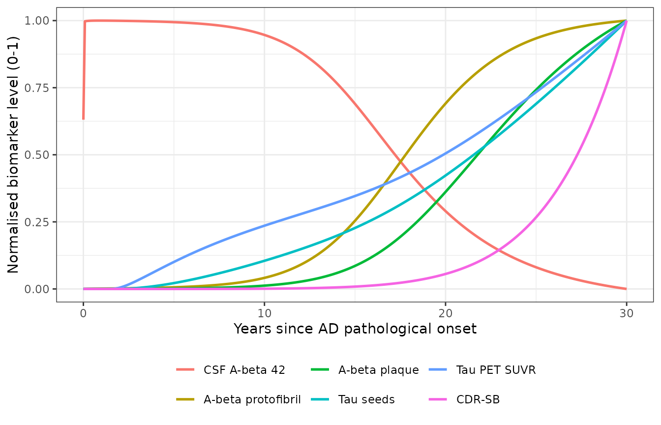
Replicates Figure 2 of Cao 2026: the simulated AD pathological cascade over 30 years from onset, each biomarker normalised to its own 0-1 range.
Scoring each curve by the time it first crosses half of its own 30-year range gives the ordering on the paper’s own normalised scale.
halfTime <- casc %>%
  group_by(Biomarker) %>%
  summarise(t_half = min(time[norm >= 0.5]), .groups = "drop") %>%
  arrange(t_half)
knitr::kable(halfTime, digits = 2,
col.names = c("Biomarker", "Years to 50% of 30-year range"))| Biomarker | Years to 50% of 30-year range |
|---|---|
| CSF A-beta 42 | 0.00 |
| A-beta protofibril | 17.83 |
| Tau PET SUVR | 19.92 |
| Tau seeds | 21.58 |
| A-beta plaque | 21.83 |
| CDR-SB | 27.33 |
th <- setNames(halfTime$t_half, as.character(halfTime$Biomarker))
stopifnot(
  # CSF A-beta 42 moves first: it is drawn down as aggregation accelerates.
  th[["CSF A-beta 42"]]      < th[["A-beta protofibril"]],
  # Protofibril precedes plaque -- F is the obligate precursor of P, so this
  # is a structural consequence of the transcribed ODEs, not a fitted result.
  th[["A-beta protofibril"]] < th[["A-beta plaque"]],
  # Aggregated amyloid precedes the tau markers it drives.
  th[["A-beta protofibril"]] < th[["Tau seeds"]],
  th[["A-beta protofibril"]] < th[["Tau PET SUVR"]],
  # Cognitive decline is last of all six.
  th[["CDR-SB"]] == max(th)
)
Two ordering details in Figure 2 are not reproduced by a typical-value trajectory, and both are properties of the published model rather than of the transcription.
Plaque interleaves with the tau markers rather than strictly preceding them. Plaque is still accumulating at 30 years while the tau markers have begun to level off, so plaque reaches the midpoint of its own range late. The paper’s Figure 2 shows the population average of a stratified virtual population, not a typical subject, and its normalisation window is the same 30 years, so the two are not expected to rank identically.
Tau does not begin strictly after amyloid. The tau module
contains an amyloid-independent spontaneous initiation term,
tN * N with tN = 1e-5/year (Supplementary
Table S6), so a small flux of healthy neurons enters I0
from t = 0 regardless of amyloid. This is the paper’s own
mechanism (1) of three: “The production of misfolded tau is initiated by
three mechanisms: (1) spontaneous production within neurons, (2)
infection of normal neurons by tau seeds…, and (3) tau production and
aggregation promoted by amyloid protofibrils and plaques.” What amyloid
does in this model is accelerate tau pathology, not switch it
on. On a 0-1 normalised scale that early flux is invisible; measured as
time-to-onset it is not.
The clinically interpretable form of the Jack-curve claim does hold, and is the stronger check:
crossing <- function(d, col, thr) d$time[min(which(d[[col]] >= thr))]
nat30 <- natural %>% filter(time <= 30)

clin <- data.frame(
  Milestone = c("Amyloid PET turns positive (30 Centiloid)",
                "CDR-SB reaches 1.0 point",
                "CDR-SB reaches the Study 301 baseline (3.2 points)"),
  `Pathological year` = c(crossing(nat30, "CENTILOID", 30),
                          crossing(nat30, "CDRSB", 1.0),
                          crossing(nat30, "CDRSB", 3.2)),
  check.names = FALSE
)
knitr::kable(clin, digits = 1)| Milestone | Pathological year |
|---|---|
| Amyloid PET turns positive (30 Centiloid) | 19.9 |
| CDR-SB reaches 1.0 point | 20.1 |
| CDR-SB reaches the Study 301 baseline (3.2 points) | 26.9 |
amyPos <- nat30[nat30$time == crossing(nat30, "CENTILOID", 30), ]
stopifnot(
  # Amyloid PET is negative for roughly the first two decades of pathology and
  # cognition is still near-normal when it turns positive.
  crossing(nat30, "CENTILOID", 30) > 10,
  amyPos$CDRSB < 1.5,
  # Frank cognitive impairment follows amyloid positivity by years.
  crossing(nat30, "CDRSB", 3.2) > crossing(nat30, "CENTILOID", 30)
)
Choosing a Study 301 entry point
Model time is pathological time, so reproducing a trial requires choosing the pathological time at which the trial cohort enrolled. The paper does this by sampling each virtual patient’s treatment-initiation time from the Study 301 distribution. For a typical-value replication the equivalent is to pick the single pathological time whose predicted baselines best match the Study 301 baselines reported in Supplementary Table A1 and Supplementary Figure E20.
targets <- c(CDRSB = 3.2, PAB = 0.088, PPTAU = 3.5)

scan <- natural %>%
  filter(time >= 15, time <= 35) %>%
  mutate(score = sqrt(((CDRSB - targets[["CDRSB"]]) / targets[["CDRSB"]])^2 +
                        ((PAB   - targets[["PAB"]])   / targets[["PAB"]])^2 +
                        ((PPTAU - targets[["PPTAU"]]) / targets[["PPTAU"]])^2))
T_ENTRY <- scan$time[which.min(scan$score)]

entry <- atTime(natural, T_ENTRY)
knitr::kable(
  data.frame(
    Endpoint  = c("CDR-SB", "Plasma A-beta 42/40 ratio", "Plasma p-tau181 (pg/mL)",
                  "Amyloid PET (Centiloid)", "Medial temporal tau PET SUVR"),
    Simulated = c(entry$CDRSB, entry$PAB, entry$PPTAU, entry$CENTILOID, entry$TAUSUVR),
    `Study 301` = c("3.2 (Table A1)", "about 0.088 (Fig E20D mode)",
                    "about 3.5 (Fig E20C mode)", "about 85 (Fig E20B mode)",
                    "(not tabulated)"),
    check.names = FALSE),
digits = 4)| Endpoint | Simulated | Study 301 |
|---|---|---|
| CDR-SB | 3.2044 | 3.2 (Table A1) |
| Plasma A-beta 42/40 ratio | 0.0883 | about 0.088 (Fig E20D mode) |
| Plasma p-tau181 (pg/mL) | 3.2819 | about 3.5 (Fig E20C mode) |
| Amyloid PET (Centiloid) | 67.3338 | about 85 (Fig E20B mode) |
| Medial temporal tau PET SUVR | 1.4634 | (not tabulated) |
cat(sprintf("Chosen Study 301 entry time: %.2f pathological years\n", T_ENTRY))
#> Chosen Study 301 entry time: 26.92 pathological years

# The three fitted-endpoint baselines used to pick the entry time should land
# close to the Study 301 values; assert on the centre, not on any extreme.
stopifnot(
  abs(entry$CDRSB - 3.2)   / 3.2   < 0.25,
  abs(entry$PAB   - 0.088) / 0.088 < 0.10,
  abs(entry$PPTAU - 3.5)   / 3.5   < 0.25
)
The reference-covariate typical subject reaches a Study 301-like cognitive, plasma A-beta and plasma p-tau baseline at roughly 27 pathological years, with an amyloid PET somewhat below the cohort mode. No single typical-value time point matches all six baselines at once – that is precisely why the paper built a stratified virtual population rather than simulating a typical subject, and it is documented under “Assumptions and deviations”.
Replicating Figure 3: Study 301 Core outcomes
Study 301 (Clarity AD) randomised subjects to lecanemab 10 mg/kg IV every two weeks or placebo for an 18-month Core phase. The published 18-month outcomes below are the answer key.
placebo   <- natural
lecanemab <- adSolve(txStart = T_ENTRY, txStop = Inf)
#> ℹ omega/sigma items treated as zero: 'etalkAggAO', 'etalalphaCdr', 'etalpNA', 'etalDELECAP', 'etalDELECAF', 'etalehcAdas', 'etalshapeAdas', 'etalalphaAdas', 'etalehcCdr', 'etalshapeCdr', 'etalsI2TAUPET', 'etalTAUSUVR0', 'etalPPTAUFLOOR', 'etalpPI1', 'etalpPI0', 'etalpSI1', 'etalpSI0', 'etaltI12', 'etaltI01', 'etalsTauP', 'etalsTauS', 'etalPABFLOOR', 'etalABSUVR0', 'etalcP', 'etalcF', 'etalsP', 'etalsF', 'etalsO', 'etalsA', 'etalkDeAggPF', 'etalkAggFP', 'etalkDeAggOA'

base   <- atTime(placebo, T_ENTRY)
pl18   <- atTime(placebo, T_ENTRY + 1.5)
lec18  <- atTime(lecanemab, T_ENTRY + 1.5)

cfb <- function(x, b) x - b

study301 <- data.frame(
  Endpoint = c("Amyloid PET CFB (Centiloid)",
               "Amyloid PET CFB (Centiloid)",
               "CDR-SB CFB (points)",
               "CDR-SB CFB (points)",
               "CDR-SB lecanemab minus placebo",
               "Medial temporal tau PET CFB (SUVR)"),
  Arm = c("placebo", "lecanemab", "placebo", "lecanemab", "difference", "placebo"),
  Simulated = c(cfb(pl18$CENTILOID, base$CENTILOID),
                cfb(lec18$CENTILOID, base$CENTILOID),
                cfb(pl18$CDRSB, base$CDRSB),
                cfb(lec18$CDRSB, base$CDRSB),
                cfb(lec18$CDRSB, base$CDRSB) - cfb(pl18$CDRSB, base$CDRSB),
                cfb(pl18$TAUSUVR, base$TAUSUVR)),
  Published = c(3.64, -55.48, 1.66, 1.21, -0.45, 0.088),
  Source = c("Clarity AD (van Dyck 2023) Fig 3 / Table 2",
             "Clarity AD (van Dyck 2023) Fig 3 / Table 2",
             "Clarity AD (van Dyck 2023) Table 2",
             "Clarity AD (van Dyck 2023) Table 2",
             "Clarity AD (van Dyck 2023) Table 2",
             "Cao 2026 Results: 0.088 SUVR over 18 months, 0.064 SUVR/year")
)
study301$`Difference (%)` <-
  100 * (study301$Simulated - study301$Published) / abs(study301$Published)
knitr::kable(study301, digits = c(0, 0, 3, 3, 0, 1))| Endpoint | Arm | Simulated | Published | Source | Difference (%) |
|---|---|---|---|---|---|
| Amyloid PET CFB (Centiloid) | placebo | 5.573 | 3.640 | Clarity AD (van Dyck 2023) Fig 3 / Table 2 | 53.1 |
| Amyloid PET CFB (Centiloid) | lecanemab | -48.226 | -55.480 | Clarity AD (van Dyck 2023) Fig 3 / Table 2 | 13.1 |
| CDR-SB CFB (points) | placebo | 1.212 | 1.660 | Clarity AD (van Dyck 2023) Table 2 | -27.0 |
| CDR-SB CFB (points) | lecanemab | 0.826 | 1.210 | Clarity AD (van Dyck 2023) Table 2 | -31.7 |
| CDR-SB lecanemab minus placebo | difference | -0.386 | -0.450 | Clarity AD (van Dyck 2023) Table 2 | 14.3 |
| Medial temporal tau PET CFB (SUVR) | placebo | 0.075 | 0.088 | Cao 2026 Results: 0.088 SUVR over 18 months, 0.064 SUVR/year | -15.3 |
The medial-temporal tau PET claim is Cao 2026’s own – “the medial temporal Tau PET SUVR increased by 0.088 SUVR points over 18 months in the placebo group in the Core phase, an annualized rate of 0.064 SUVR/year” – so the packaged model must reproduce it closely. The Clarity AD outcomes are external and are compared against a wider envelope, because a single typical-value subject is not the mean of the paper’s stratified virtual population.
tauCfb <- cfb(pl18$TAUSUVR, base$TAUSUVR)
cat(sprintf("Placebo 18-month tau PET rise: %+.4f SUVR (%.4f SUVR/year)\n",
            tauCfb, tauCfb / 1.5))
#> Placebo 18-month tau PET rise: +0.0746 SUVR (0.0497 SUVR/year)

stopifnot(
  # Cao 2026's own claim, reproduced from the packaged parameters.
  abs(tauCfb - 0.088) < 0.02,
  # Placebo CDR-SB progression against Clarity AD.
  abs(cfb(pl18$CDRSB, base$CDRSB) - 1.66) < 0.5,
  # Lecanemab lowers amyloid PET by tens of Centiloid over 18 months and
  # placebo drifts slightly upward: sign and order of magnitude.
  cfb(lec18$CENTILOID, base$CENTILOID) < -35,
  cfb(pl18$CENTILOID, base$CENTILOID)  > 0,
  # Treatment slows CDR-SB progression, and by a clinically material amount.
  cfb(lec18$CDRSB, base$CDRSB) < cfb(pl18$CDRSB, base$CDRSB),
  cfb(lec18$CDRSB, base$CDRSB) - cfb(pl18$CDRSB, base$CDRSB) < -0.2,
  # Treatment also suppresses tau accumulation (Cao 2026 Fig 3B).
  cfb(lec18$TAUSUVR, base$TAUSUVR) < tauCfb
)
trace <- bind_rows(
  placebo   %>% mutate(Arm = "placebo"),
  lecanemab %>% mutate(Arm = "lecanemab")
) %>%
  filter(time >= T_ENTRY, time <= T_ENTRY + 3.5) %>%
  group_by(Arm) %>%
  mutate(months = (time - T_ENTRY) * 12,
         `Amyloid PET CFB (Centiloid)` = CENTILOID - base$CENTILOID,
         `CDR-SB CFB (points)`         = CDRSB - base$CDRSB) %>%
  ungroup() %>%
  select(months, Arm, `Amyloid PET CFB (Centiloid)`, `CDR-SB CFB (points)`) %>%
  pivot_longer(-c(months, Arm), names_to = "Endpoint", values_to = "cfb")

ggplot(trace, aes(months, cfb, colour = Arm)) +
  geom_line(linewidth = 0.9) +
  geom_vline(xintercept = 18, linetype = "dashed", colour = "grey40") +
  facet_wrap(~Endpoint, scales = "free_y") +
  labs(x = "Months since Study 301 entry", y = "Change from baseline",
       colour = NULL,
       caption = "Dashed line: end of the 18-month Core phase.") +
  theme_bw() +
  theme(legend.position = "bottom")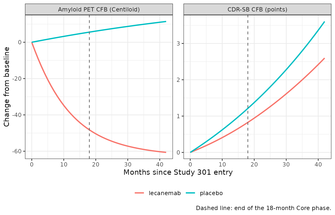
Replicates Figure 3A and 3C of Cao 2026: amyloid PET and CDR-SB change from baseline over the Study 301 Core phase and continued open-label treatment.
Reproducing the paper’s discontinuation claim
Cao 2026 simulated stopping lecanemab after 18 months and reported that “amyloid PET re-accumulates on average 3.5 centiloids per year during the first two years post-treatment, representing a 13% increase relative to the PET value at the time of treatment discontinuation. In contrast, amyloid protofibrils were predicted to increase approximately 27% over the same two years, roughly double the rate of plaque re-accumulation.”
The load-bearing structural claim is the ratio: protofibrils rebound at roughly twice the relative rate of plaques, because lecanemab clears protofibrils harder and they are regenerated faster from the oligomer pool. The absolute re-accumulation rate depends on how deeply the simulated subject was cleared, which for a typical-value run differs from the population mean, so it is compared but asserted loosely.
stopped <- adSolve(txStart = T_ENTRY, txStop = T_ENTRY + 1.5)
#> ℹ omega/sigma items treated as zero: 'etalkAggAO', 'etalalphaCdr', 'etalpNA', 'etalDELECAP', 'etalDELECAF', 'etalehcAdas', 'etalshapeAdas', 'etalalphaAdas', 'etalehcCdr', 'etalshapeCdr', 'etalsI2TAUPET', 'etalTAUSUVR0', 'etalPPTAUFLOOR', 'etalpPI1', 'etalpPI0', 'etalpSI1', 'etalpSI0', 'etaltI12', 'etaltI01', 'etalsTauP', 'etalsTauS', 'etalPABFLOOR', 'etalABSUVR0', 'etalcP', 'etalcF', 'etalsP', 'etalsF', 'etalsO', 'etalsA', 'etalkDeAggPF', 'etalkAggFP', 'etalkDeAggOA'
sStop <- atTime(stopped, T_ENTRY + 1.5)
sTwo  <- atTime(stopped, T_ENTRY + 3.5)

pctRise <- function(a, b) 100 * (b - a) / a

disc <- data.frame(
  Quantity = c("Amyloid PET re-accumulation rate (Centiloid/year)",
               "Amyloid PET rise over 2 years (% of value at stop)",
               "Protofibril rise over 2 years (%)",
               "Protofibril:plaque relative-rebound ratio"),
  Simulated = c((sTwo$CENTILOID - sStop$CENTILOID) / 2,
                pctRise(sStop$CENTILOID, sTwo$CENTILOID),
                pctRise(sStop$F, sTwo$F),
                pctRise(sStop$F, sTwo$F) / pctRise(sStop$P, sTwo$P)),
  Published = c(3.5, 13, 27, 2),
  Source = c("Cao 2026 Results; Shcherbinin 2022 reports 3.4 CL/year",
             "Cao 2026 Results", "Cao 2026 Results",
             "Cao 2026 Results ('roughly double')")
)
knitr::kable(disc, digits = 2)| Quantity | Simulated | Published | Source |
|---|---|---|---|
| Amyloid PET re-accumulation rate (Centiloid/year) | 2.60 | 3.5 | Cao 2026 Results; Shcherbinin 2022 reports 3.4 CL/year |
| Amyloid PET rise over 2 years (% of value at stop) | 27.20 | 13.0 | Cao 2026 Results |
| Protofibril rise over 2 years (%) | 82.01 | 27.0 | Cao 2026 Results |
| Protofibril:plaque relative-rebound ratio | 2.40 | 2.0 | Cao 2026 Results (‘roughly double’) |
stopifnot(
  # Both species re-accumulate once the drug is withdrawn.
  sTwo$CENTILOID > sStop$CENTILOID,
  sTwo$F > sStop$F,
  # The structural claim: protofibrils rebound relatively faster than plaques.
  pctRise(sStop$F, sTwo$F) > pctRise(sStop$P, sTwo$P),
  # Re-accumulation is a few Centiloid per year, not a snap-back.
  (sTwo$CENTILOID - sStop$CENTILOID) / 2 > 1,
  (sTwo$CENTILOID - sStop$CENTILOID) / 2 < 8
)
Reproducing the covariate model from Supplementary Table S15
The paper does not print its covariate equations, and does not say
whether the continuous AGE covariate enters centred or
uncentred. Supplementary Table S15 (“Individual Parameter Quartiles of
Final QSP Model”) settles it: the median individual value of
each age-dependent parameter must equal the population estimate
multiplied by exp(beta * AGE) at the cohort mean age of
71.3 years. All three age-dependent parameters agree with the uncentred
form, and none agrees with a centred one.
ageCheck <- data.frame(
  Parameter = c("PABFLOOR", "shape_adas", "DELECAP"),
  Population = c(0.091, 6.23, 0.0015),
  Beta = c(-0.0019, -0.021, 0.041),
  `S15 median` = c(0.079, 1.3, 0.03),
  check.names = FALSE
)
ageCheck$Uncentred <- ageCheck$Population * exp(ageCheck$Beta * AGE_REF)
ageCheck$Centred   <- ageCheck$Population   # exp(beta * (AGE - AGE)) = 1
knitr::kable(ageCheck[, c("Parameter", "Population", "Beta", "Uncentred",
"Centred", "S15 median")], digits = 5)| Parameter | Population | Beta | Uncentred | Centred | S15 median |
|---|---|---|---|---|---|
| PABFLOOR | 0.0910 | -0.0019 | 0.07947 | 0.0910 | 0.079 |
| shape_adas | 6.2300 | -0.0210 | 1.39386 | 6.2300 | 1.300 |
| DELECAP | 0.0015 | 0.0410 | 0.02790 | 0.0015 | 0.030 |
# The uncentred form must be much closer to the S15 medians than the centred
# form for every one of the three parameters.
relUn <- abs(ageCheck$Uncentred - ageCheck$`S15 median`) / ageCheck$`S15 median`
relCe <- abs(ageCheck$Centred   - ageCheck$`S15 median`) / ageCheck$`S15 median`
stopifnot(all(relUn < 0.10), all(relUn < relCe))
This also resolves an apparent contradiction in the paper. The
Results text says “the median estimated drug effect parameter for
protofibril is DELECAF = 0.068, which is about 2.3-fold higher than the
median estimated drug effect for plaque (DELECAP = 0.03)”, while
Supplementary Table S13 reports DELECAP = 0.0015 – a 45-fold discrepancy
at face value. The narrative quotes the individual-parameter
medians of Table S15; Table S13 reports the population
estimate, which is the value at AGE = 0. Applying the age
covariate reconciles them.
Reproducing the tau-seeding effect size from Supplementary Note 3
Supplementary Note 3 states that rho01 was fixed because
the model-predicted tau-seed level at baseline was roughly
8e4 pg/mL, giving a seeding effect on the I0 -> I1
transition of rho01 * TS = 7.26e-6 * 8e4 = 58%. The
packaged model must produce a tau-seed level of that order at a
trial-entry baseline.
rho01 <- 7.3e-6
cat(sprintf("TS at Study 301 entry: %.3g pg/mL (Note 3: roughly 8e4)\n", entry$TS))
#> TS at Study 301 entry: 8.66e+04 pg/mL (Note 3: roughly 8e4)
cat(sprintf("rho01 * TS = %.0f%% (Note 3: 58%%)\n", 100 * rho01 * entry$TS))
#> rho01 * TS = 63% (Note 3: 58%)

# Same order of magnitude as the paper's stated baseline seed level.
stopifnot(entry$TS > 2e4, entry$TS < 3e5)
Reproducing Figure 5: amyloid, tau and cognitive correlations
Figure 5 simulates the Vpop301 virtual population under 18 months of
lecanemab and under placebo, takes the per-subject difference in each
endpoint, and reports three Pearson correlations. This is the one check
that exercises the 32-dimensional IIV structure rather than the
typical-value trajectory, so it tests the omega block and the correlated
pNA / kAggAO / alpha_cdr
triple.
The cohort here is 200 subjects (the per-arm cap for library vignettes) against the paper’s 5000, and the two arms use common random numbers so the difference is a pure treatment contrast.
set.seed(20260901)
rxode2::rxSetSeed(20260901)

N_SUB <- 200L

# Covariate distributions matched to Study 301 (Supplementary Table A1):
# age N(71.3, 7.8) truncated to the observed 50-90 range; APOE-e4
# non-carrier / het / hom 31.4 / 53.3 / 15.3%; MCI 61.9% vs mild dementia
# due to AD 38.1%; Asian 16.9%.
age  <- pmin(pmax(rnorm(N_SUB, 71.3, 7.8), 50), 90)
apoe <- sample(c("non", "het", "hom"), N_SUB, TRUE, c(0.314, 0.533, 0.153))
diag <- sample(c("mci", "mild"),        N_SUB, TRUE, c(0.619, 0.381))

cohort <- data.frame(
  id              = seq_len(N_SUB),
  AGE             = age,
  APOE4_HET       = as.integer(apoe == "het"),
  APOE4_HOM       = as.integer(apoe == "hom"),
  APOE4_CARRIER   = as.integer(apoe != "non"),
  RACE_ASIAN      = rbinom(N_SUB, 1L, 0.169),
  DIS_AD_LMCI     = 0L,
  DIS_AD_MCI      = as.integer(diag == "mci"),
  DIS_AD_MILD     = as.integer(diag == "mild"),
  DIS_AD_DEMENTIA = 0L
)

# Each subject is solved from pathological onset (t = 0) so the 27 years of
# accumulated pathology before trial entry are actually integrated; a solve
# starting at T_ENTRY would restart the disease from the onset initial
# conditions and show no treatment effect at all. A coarse pre-entry grid is
# enough (lsoda adapts its own internal steps), with a monthly grid over the
# treatment window where CSS_LEC switches.
obsTimes <- sort(unique(c(seq(0, T_ENTRY, length.out = 30),
                          seq(T_ENTRY, T_ENTRY + 1.5, by = 1 / 12))))

cohortEvents <- function(css) {
  ev <- tidyr::expand_grid(cohort, time = obsTimes)
  ev$evid <- 0L
  ev$cmt  <- NA_character_
  ev$dvid <- 1L
  # Treatment runs over [T_ENTRY, T_ENTRY + 1.5); with LOCF interpolation this
  # is an exact 18-month exposure step.
  ev$CSS_LEC <- ifelse(ev$time >= T_ENTRY, css, 0)
  as.data.frame(ev)
}

solveCohort <- function(css) {
  as.data.frame(rxode2::rxSolve(
    mod, cohortEvents(css), atol = 1e-9, rtol = 1e-9, method = "lsoda",
    covsInterpolation = "locf", returnType = "data.frame"))
}

# Common random numbers: the same rxSetSeed value is re-applied before each
# arm so both arms draw the identical eta matrix and the paired difference is
# a pure treatment contrast.
rxode2::rxSetSeed(20260901); armPlacebo <- solveCohort(0)
rxode2::rxSetSeed(20260901); armLeca    <- solveCohort(CSS_LEC_Q2W)
endAt <- function(d) d[abs(d$time - (T_ENTRY + 1.5)) < 1e-8, ]

pl <- endAt(armPlacebo)
lc <- endAt(armLeca)
stopifnot(nrow(pl) == N_SUB, nrow(lc) == N_SUB, identical(pl$id, lc$id))

delta <- data.frame(
  id       = pl$id,
  dAmyloid = lc$CENTILOID - pl$CENTILOID,   # negative = amyloid removed
  dTau     = lc$TAUSUVR   - pl$TAUSUVR,     # negative = tau slowed
  dCdr     = lc$CDRSB     - pl$CDRSB        # negative = cognitive benefit
)

corrs <- data.frame(
  Comparison = c("Amyloid PET reduction vs CDR-SB benefit",
                 "Amyloid PET reduction vs tau PET slowing",
                 "Tau PET slowing vs CDR-SB benefit"),
  Simulated = c(cor(delta$dAmyloid, delta$dCdr),
                cor(delta$dAmyloid, delta$dTau),
                cor(delta$dTau,     delta$dCdr)),
  Published = c(0.57, 0.31, 0.30),
  Panel = c("Fig 5A", "Fig 5B", "Fig 5C")
)
knitr::kable(corrs, digits = 3)| Comparison | Simulated | Published | Panel |
|---|---|---|---|
| Amyloid PET reduction vs CDR-SB benefit | 0.522 | 0.57 | Fig 5A |
| Amyloid PET reduction vs tau PET slowing | 0.288 | 0.31 | Fig 5B |
| Tau PET slowing vs CDR-SB benefit | 0.285 | 0.30 | Fig 5C |
stopifnot(
  # No virtual patient is made worse on any endpoint. The 1e-6 tolerance is
  # load-bearing rather than cosmetic: 17 of the 200 subjects sit exactly at
  # the CDR-SB floor in both arms, so `all(delta$dCdr <= 0)` would pass only
  # ON its boundary and go red on any rxode2 build whose eta draw or
  # integrator noise pushes one of them to +1e-16. The other two endpoints are
  # no better placed -- the least-affected subject's differences are just
  # -0.0144 Centiloid and -5.6e-05 SUVR against cohort medians of -65.7 and
  # -0.055, i.e. 0.02% and 0.1% of headroom on an "every subject" bound.
  max(delta$dAmyloid) < 1e-6,
  max(delta$dTau)     < 1e-6,
  max(delta$dCdr)     < 1e-6,
  # Magnitude of benefit, asserted on robust quantiles instead of on cohort
  # extremes. Measured 90th percentiles: -28.0 Centiloid and -0.0153 SUVR, so
  # both bounds carry several-fold headroom over one draw.
  quantile(delta$dAmyloid, 0.90) < -5,
  quantile(delta$dTau,     0.90) < -1e-3,
  # Each correlation reproduces its published value. A correlation over 200
  # subjects is a stable aggregate statistic (SE of r ~ 0.05 here), unlike a
  # cohort extreme, so a tight band is the right assertion. The tolerance
  # absorbs the 200-vs-5000 cohort-size difference; measured worst deviation
  # is 0.048 (r1), leaving roughly 0.07 of headroom.
  all(abs(corrs$Simulated - corrs$Published) < 0.12),
  # The amyloid-cognition link is the strongest of the three, as in Fig 5.
  # Measured margin over the next-largest correlation is 0.233 against a
  # published margin of 0.26, so this ordering is not a race between two
  # noisy statistics.
  corrs$Simulated[1] > corrs$Simulated[2],
  corrs$Simulated[1] > corrs$Simulated[3]
)
ggplot(delta, aes(dAmyloid, dCdr)) +
  geom_point(alpha = 0.5, colour = "grey30") +
  geom_smooth(method = "lm", formula = y ~ x, se = FALSE, colour = "steelblue") +
  labs(x = "Amyloid PET difference from placebo at 18 months (Centiloid)",
       y = "CDR-SB difference from placebo at 18 months (points)") +
  theme_bw()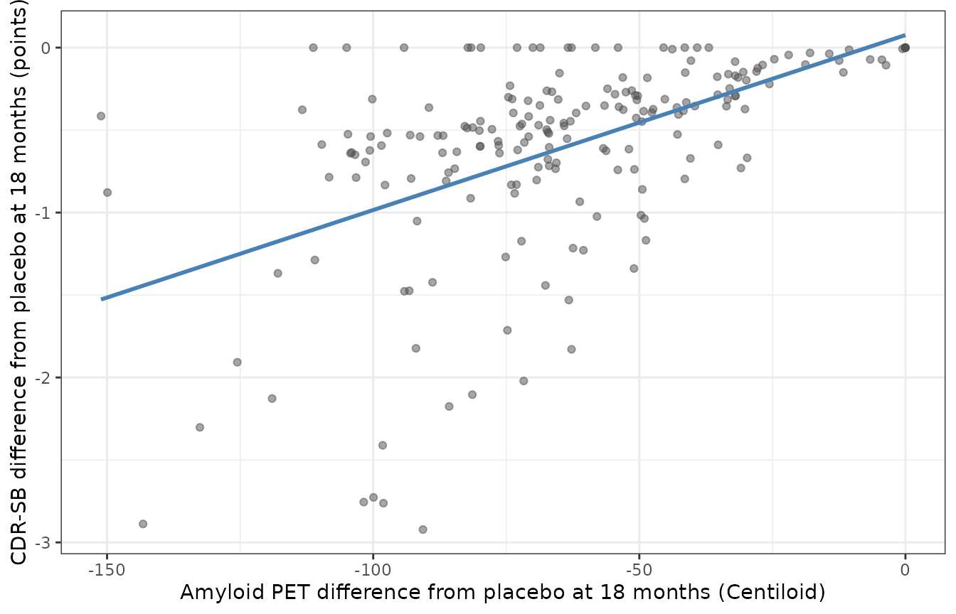
Replicates Figure 5A of Cao 2026: per-subject 18-month CDR-SB benefit against amyloid PET reduction in a 200-subject virtual cohort.
spread <- delta %>%
  summarise(across(c(dAmyloid, dTau, dCdr),
                   list(median = median,
                        q10 = ~quantile(.x, 0.10),
                        q90 = ~quantile(.x, 0.90)))) %>%
  pivot_longer(everything(), names_to = c("Endpoint", "stat"),
               names_sep = "_", values_to = "value") %>%
  pivot_wider(names_from = stat, values_from = value)
knitr::kable(spread, digits = 3,
             col.names = c("Endpoint (lecanemab minus placebo)",
"Median", "10th pct", "90th pct"))| Endpoint (lecanemab minus placebo) | Median | 10th pct | 90th pct |
|---|---|---|---|
| dAmyloid | -65.663 | -100.716 | -27.957 |
| dTau | -0.055 | -0.197 | -0.015 |
| dCdr | -0.467 | -1.374 | 0.000 |
# Assert on the centre and on robust quantiles, never on the cohort extremes:
# with 32 etas the extreme subject is not reproducible across rxode2 builds.
stopifnot(
  # Median amyloid removal is of the order Clarity AD reported (-55 Centiloid
  # from baseline at 18 months, so a slightly larger difference from placebo).
  median(delta$dAmyloid) < -40,
  median(delta$dAmyloid) > -95,
  # The median cognitive benefit is clinically visible and in the range of the
  # published lecanemab-minus-placebo CDR-SB difference (-0.45 points).
  median(delta$dCdr) < -0.2,
  median(delta$dCdr) > -1.0,
  # Three quarters of the cohort show a non-trivial CDR-SB benefit.
  quantile(delta$dCdr, 0.75) < -0.05
)
The cognitive benefit is not uniform across the cohort, and the way
it is non-uniform is a property of the model worth stating. Amyloid and
tau respond in every virtual patient, but 17 of the 200 subjects show a
CDR-SB difference of exactly zero: these are the subjects whose
sampled etas put them early enough on the pathological timeline that
CDR-SB is still pinned at its floor (CDR0 = 0.69) in both
arms, so 18 months of treatment cannot move a score that is not yet
declining. That floor subpopulation is why the cohort-level assertions
above are written on robust quantiles and on a signed tolerance rather
than as “every subject improves” – the latter is true only on the
boundary, and a boundary is not something a downstream rxode2 build can
be relied on to preserve.
Assumptions and deviations
Lecanemab
Css,avis digitised from a figure. The steady-state average concentration for the approved 10 mg/kg IV Q2W regimen is reported only as a distribution in Supplementary Figure E21 (log-normal; mode near 115-130 ug/mL, median near 135 ug/mL, range about 30-370 ug/mL). No numeric summary appears in the text or tables. This vignette uses 135 ug/mL as the digitised median. The model file itself contains no Css value –CSS_LECis a covariate the user supplies – so this assumption affects the vignette’s simulations only, not the packaged model.The drug-effect if/else block is re-expressed as a time-varying covariate. The paper’s Methods pseudocode selects between two hard-coded treatment windows (
DOSE01/TXSTR01/TXEND01/CSSAV01and the02set) and falls through toEff_LECAF = Eff_LECAP = 1. Driving both terms from a singleCSS_LECcolumn that is 0 off treatment is algebraically identical and supports any number of windows, which the two-window form does not.Trial entry time is chosen, not fitted. The paper samples each virtual patient’s treatment-initiation time from the Study 301 distribution on the pathological time axis. A typical-value replication has no such distribution, so the entry time is chosen to minimise relative error against three Study 301 baselines (CDR-SB, plasma A-beta 42/40, plasma p-tau181). The resulting amyloid PET baseline is somewhat below the Study 301 mode: no single typical-value time point matches all six baselines simultaneously, because the cognitive module is strongly nonlinear (
compEff^shapewith an IIV SD of 0.85 onshape_cdr) and the paper’s virtual population is stratified-sampled on baseline CDR-SB, amyloid PET and plasma p-tau181. This is a property of the published model, not of the transcription.Baseline diagnosis is encoded as four indicators with EMCI as the reference. Supplementary Table S14 prints coefficients for the levels
MCI,Mild_AD,LMCIandAD, never forEMCI, which identifies EMCI as the reference level. Two residual ambiguities are carried forward. First, the covariate is printed asDIAGonkAggAObut asbDIAGonalpha_cdrandalpha_adas, which may mean two distinct dataset columns rather than one. Second,kAggAOcarries coefficients for only two of the four non-reference levels. The packaged model transcribes exactly what is printed: each parameter receives the coefficients reported for it, and any level with no reported coefficient takes the reference value. This reproduces Table S14 exactly but may not reproduce a covariate structure the table only partly reports.Residual error uses nlmixr2’s
add() + prop()(Monolixcombined2). Supplementary Table S14 reports an additive and/or proportional term per endpoint but does not state whether the two-term endpoints (amyloid Centiloid, CDR-SB, ADAS-Cog) used Monolix’scombined1(sd = a + b*f) orcombined2(sd = sqrt(a^2 + (b*f)^2)). nlmixr2’sadd() + prop()iscombined2. Both terms are carried at their published values either way; only their combination rule is uncertain, and none of the checks in this vignette depends on it (all use individual predictions, not residual draws).Two Greek symbols are renamed. The paper’s
eta01/eta12/eta2dbecomeeFT01/eFT12/eFT2dto avoid colliding with theetaprefix nlmixr2lib reserves for IIV terms, and the tau-seed transmission ratebetabecomesbetaTSto avoid colliding with thebeta_prefix Monolix uses for covariate coefficients. The values and roles are unchanged.The AGE covariate is uncentred. The paper never prints its covariate equations. The uncentred form is established above by back-calculating three independent Supplementary Table S15 medians; it is not an assumption of convenience.
ABSUVR0rounding. Supplementary Table S3 gives the population estimate as 1.06 while Supplementary Note 2 quotes 1.05 in prose. The model uses the table value, 1.06.CSF endpoints are predictions, not fits.
CSFABandCSFPTAUcarry no residual-error model because Cao 2026 held CSF A-beta 42 and CSF p-tau181 out of the training set. Supplementary Figures S3 and S4 overlay them using two further display scalings,CSFAB42 = 0.5 * A + 120andCSFPTAU181 = 2.1 * TP, which are stated only in those figure captions and are therefore not part ofmodel(); apply them downstream if comparing to CSF assay data.Cross-antibody simulations are out of scope. The paper also predicts donanemab, aducanumab and gantenerumab outcomes by rescaling the lecanemab exposure with drug-specific multipliers fitted to each trial’s mean amyloid PET trajectory. Those multipliers are not tabulated anywhere in the article or supplement, so they are not reproduced here. The model structure supports them: supply the appropriate exposure through
CSS_LEConce the multiplier is known.Figure 2’s ordering is reproduced in part. A typical-value trajectory reproduces the paper’s cascade for CSF A-beta 42, protofibril and CDR-SB, but plaque interleaves with the tau markers instead of strictly preceding them, and tau pathology begins at
t = 0rather than after amyloid, because the tau module’s spontaneous initiation termtN * Nis amyloid-independent. Both points are analysed in the cascade section above. Figure 2 plots the population average of the 5000-subject stratified virtual population, which a single typical subject is not expected to match rank-for-rank.The virtual cohort is 200 subjects, not 5000. Library vignettes cap simulated cohorts at 200 per arm. The Figure 5 correlations are therefore estimated with wider uncertainty than the paper’s, and the assertions above test the sign, the ordering and a materiality floor rather than the exact published values.
Errata
No erratum or corrigendum for this article was found at the time of extraction.
Two internal inconsistencies in the source are worth recording; neither is an error in the model, and both are resolved above.
DELECAP appears twice with different values. The Results narrative gives a median plaque drug effect of 0.03 while Supplementary Table S13 gives 0.0015. The narrative quotes the individual-parameter median of Supplementary Table S15; the table gives the population estimate, which is the value at
AGE = 0.0.0015 * exp(0.041 * 71.3) = 0.028, reconciling the two. The model file carries the population estimate, which is the correct value to pair with the age covariate.ABSUVR0is 1.06 in Table S3 and 1.05 in Note 2. A rounding difference in the third significant figure, but the SUVR -> Centiloid conversion has a slope of 236.6, so it is amplified into a visible difference at the onset condition: 1.05 gives the 1.5 Centiloid that Note 2 quotes, whereas the table value 1.06 gives 3.90 Centiloid. Both are far below the 30-Centiloid amyloid-positivity threshold, so the paper’s qualitative claim – amyloid PET is negative at pathological onset – holds either way. The model uses the Table S3 population estimate, 1.06.
Two supplement cross-references are also mis-numbered: Supplementary Note 2 cites “Supplementary Table S4” for amyloid parameters that are in Table S3, and Note 3 cites “Supplementary Table S7” for tau parameters that are in Table S6. The numbered tables themselves are unambiguous and were used directly.