Efaproxiral (Gastonguay 2005)
Source:vignettes/articles/Gastonguay_2005_efaproxiral.Rmd
Gastonguay_2005_efaproxiral.RmdModel and source
- Citation: Gastonguay MR, Venitz J, Steffen RP, Hackman J. Population pharmacokinetic-pharmacodynamic modeling of efaproxiral in cancer patients receiving radiation therapy. Clin Pharmacol Ther. 2005;77(2):P89 (PII-101). ASCPT 2005 annual meeting poster. doi:10.1016/j.clpt.2004.12.233.
- Description: Linear 2-compartment IV popPK model for efaproxiral (RSR13) with an algebraic linear RBC:plasma proportionality (Crbc = SLPRBC * Cc) and a linear PD model relating partial pressure of oxygen at 50% hemoglobin saturation (p50, mmHg) to RBC efaproxiral concentration (p50 = INTp50 + SLPp50 * Crbc). Population of 451 cancer patients receiving radiation therapy pooled across six phase I-III trials. Full covariate model: BSA and AGE on CL; BSA, AGE and baseline albumin (BALB) on V1 and V2; BSA on Q; max administered dose (MDOS), AGE and BALB on SLPRBC; primary cancer type indicators (breast, glioma, other; reference = lung) on SLPp50. Three-way correlated IIV block on CL, V1, V2 plus diagonal IIV on Q, SLPRBC, INTp50 and SLPp50.
- Article (open-access poster PDF): https://metrumrg.com/wp-content/uploads/2018/08/ascpt_2005_efapoxiral.pdf
- Conference abstract: Clin Pharmacol Ther 2005;77(2):P89, doi:10.1016/j.clpt.2004.12.233.
Efaproxiral (EFP, RSR13) is a synthetic allosteric modifier of hemoglobin that reduces oxygen-binding affinity (raises p50, the partial pressure of oxygen at which 50% of hemoglobin is saturated). It was investigated as a radiation- therapy sensitizer in cancer patients. The Gastonguay 2005 ASCPT poster describes the population PK-PD model fit to pooled data from six phase I-III clinical trials.
Population
The structural model was fit to 7,946 observations (2,582 plasma efaproxiral concentrations, 2,881 RBC efaproxiral concentrations, and 2,483 p50 values from the phase I-II studies only) from 451 cancer patients receiving radiation therapy (Data section). Subjects were 50.3% female with a median age of 57 years (range 28-87), median weight 72.3 kg (range 38.6-129), median BSA 1.82 m^2 (range 1.31-2.50), and median baseline serum albumin 3.6 g/dL (range 2.2-5.0). The race distribution was Caucasian 90.2%, Black 5.8%, Hispanic 2.0%, Asian 0.7%, Native American 0.2%, Other 1.1% (Table 1). Primary cancer types were lung (50.8%), breast (17.3%), cranial glioblastoma multiforme (16.0%) and other (16.0%).
Efaproxiral was administered as a 30-minute IV infusion at 75 or 100 mg/kg, 2-3 times per week. The protocol-specified dosing rule in the studies modeled was 100 mg/kg for males <= 95 kg and females <= 70 kg, and 75 mg/kg otherwise (Figure 5 caption).
The same information is available programmatically via the model’s
population metadata:
readModelDb("Gastonguay_2005_efaproxiral")()$population.
Source trace
The per-parameter origin is recorded inline next to each
ini() entry in
inst/modeldb/specificDrugs/Gastonguay_2005_efaproxiral.R.
The table below collects them in one place for reviewer audit.
| Equation / parameter | Value | Source location |
|---|---|---|
lcl (CL) |
1.88 L/h (RSE 8%) | Table 3 row “CL” |
lvc (V1) |
10.5 L (RSE 2%) | Table 3 row “V1” |
lq (Q) |
2.58 L/h (RSE 12%) | Table 3 row “Q” |
lvp (V2) |
18.1 L (RSE 10%) | Table 3 row “V2” |
lslprbc (SLPRBC) |
0.982 (RSE 1%) | Table 3 row “SLPRBC” |
lrbase_p50 (INTp50) |
26.9 mmHg (RSE ~0%) | Table 3 row “INTp50” |
lslope_p50 (SLPp50) |
0.0193 mmHg/(ug/mL) | Table 3 row “SLPp50” (RSE 5%) |
e_bsa_cl (CL~BSA) |
0.528 (RSE 101%) | Table 3, Equation 1 |
e_age_cl (CL~AGE) |
-1.0 (RSE 25%) | Table 3, Equation 1 |
e_bsa_vc (V1~BSA) |
1.15 (RSE 11%) | Table 3, Equation 1 |
e_age_vc (V1~AGE) |
-0.282 (RSE 27%) | Table 3, Equation 1 |
e_alb_vc (V1~BALB) |
0.357 (RSE 47%) | Table 3, Equation 1 |
e_bsa_q (Q~BSA) |
0.199 (RSE 426%) | Table 3, Equation 1 |
e_bsa_vp (V2~BSA) |
2.62 (RSE 29%) | Table 3, Equation 1 |
e_age_vp (V2~AGE) |
0.524 (RSE 81%) | Table 3, Equation 1 |
e_alb_vp (V2~BALB) |
-2.35 (RSE 57%) | Table 3, Equation 1 |
e_dose_efp_max_slprbc |
-0.125 (RSE 42%) | Table 3, Equation 1 |
e_age_slprbc |
-0.109 (RSE 49%) | Table 3, Equation 1 |
e_alb_slprbc |
0.367 (RSE 38%) | Table 3, Equation 1 |
e_breast_slope_p50 |
log(1.11) (RSE 8%) | Table 3, Equation 1 (CATP=2 multiplier) |
e_glio_slope_p50 |
log(1.28) (RSE 18%) | Table 3, Equation 1 (CATP=3 multiplier) |
e_other_slope_p50 |
log(0.854) (RSE 11%) | Table 3, Equation 1 (CATP=4 multiplier) |
| Reference values | BSA=1.8 m^2, AGE=60 yr, BALB=3.5 g/dL, MDOS=6800 mg | Equation 1 denominators |
| Omega^2 block (CL, V1, V2) | diag = 0.283, 0.0324, 4.66; off-diag = 0.0264, -0.41, 0.0341 | Table 3 plus footnotes a, b, c |
| Omega^2 (Q) | 0.154 (CV% 39%) | Table 3 row “Q” |
| Omega^2 (SLPRBC) | 0.0176 (CV% 13%) | Table 3 row “SLPRBC” |
| Omega^2 (INTp50) | 0.00217 (CV% 5%) | Table 3 row “INTp50” |
| Omega^2 (SLPp50) | 0.0568 (CV% 24%) | Table 3 row “SLPp50” |
| Plasma additive SD | 24.74 ug/mL (RSE 26%) | Table 3 “Residual Error” block |
| Plasma proportional SD | 12.96% (RSE 11%) | Table 3 “Residual Error” block |
| RBC additive SD | 15.62 ug/mL (RSE 27%) | Table 3 “Residual Error” block |
| RBC proportional SD | 15.56% (RSE 15%) | Table 3 “Residual Error” block |
| p50 proportional SD | 6.86% (RSE 18%) | Table 3 “Residual Error” block |
d/dt(central) = ... |
Linear 2-compartment | Equation 1 PK block (“Run 332” goodness-of-fit) |
Crbc = slprbc * Cc |
Algebraic | Equation 1 (“RBC concentration” line) |
p50 = INTp50 + SLPp50 * Crbc |
Linear PD | Equation 1 (“p50” line) |
Virtual cohort
The original observed data are not publicly available. The simulation below uses a virtual cohort whose covariate distributions approximate the demographics reported in Gastonguay 2005 Table 1. The per-protocol dosing rule from Figure 5 (100 mg/kg for “small” patients, 75 mg/kg for “large” patients) is applied.
set.seed(20050204) # ASCPT 2005 meeting

n_per_arm <- 100L

# Helper: simulate a virtual subject with the paper's per-protocol dosing rule
# encoded so the assigned dose is determined by sex and weight thresholds.
make_cohort <- function(n, cancer_type, id_offset = 0L) {
  # Sex: ~50% female (paper Table 1: 49.7% male, 50.3% female).
  sex_f <- rbinom(n, 1, 0.503)

  # Weight: lognormal centered on median 72.3 kg, truncated to [38.6, 129].
  wt <- pmax(38.6, pmin(129, exp(rnorm(n, log(72.3), 0.18))))

  # Height: approximate cohort median 169 cm, range 135-193.
  ht <- pmax(135, pmin(193, rnorm(n, 169, 9.5)))

  # BSA via Du Bois formula (m^2). Reasonable approximation matching the
  # cohort median 1.82 m^2 (range 1.31-2.50).
  bsa <- 0.007184 * (wt^0.425) * (ht^0.725)
  bsa <- pmax(1.31, pmin(2.50, bsa))

  # Age: median 57 (range 28-87); truncated normal.
  age <- pmax(28, pmin(87, round(rnorm(n, 57, 12))))

  # Baseline albumin: median 3.6 g/dL (range 2.2-5.0). Stored in SI g/L
  # for the canonical ALB column; the model converts back to g/dL inline.
  alb_gdL <- pmax(2.2, pmin(5.0, rnorm(n, 3.6, 0.5)))
  alb_gL  <- alb_gdL * 10

  # Per-protocol dosing rule (Figure 5 caption):
  #   100 mg/kg for males <= 95 kg and females <= 70 kg;
  #    75 mg/kg otherwise.
  dose_per_kg <- ifelse(sex_f == 0 & wt <= 95, 100,
                 ifelse(sex_f == 1 & wt <= 70, 100, 75))
  dose_mg <- dose_per_kg * wt
  # MDOS column (per-subject maximum administered dose, mg) equals the
  # per-protocol single dose in this single-dose simulation.
  mdos <- dose_mg

  # Categorical cancer-type indicators. CATP=1 (lung) is the implicit
  # reference (all three indicators = 0).
  cat_breast <- as.integer(cancer_type == "breast")
  cat_glio   <- as.integer(cancer_type == "glio")
  cat_other  <- as.integer(cancer_type == "other")

  tibble(
    id              = id_offset + seq_len(n),
    WT              = wt,
    HT              = ht,
    BSA             = bsa,
    AGE             = age,
    ALB             = alb_gL,
    SEXF            = sex_f,
    DOSE_EFP_MAX_MG = mdos,
    TUMTP_BREAST    = cat_breast,
    TUMTP_GLIO      = cat_glio,
    TUMTP_OTHER     = cat_other,
    dose_mg         = dose_mg,
    cancer_type     = cancer_type
  )
}

# Build a single-cohort vignette using the largest cohort (lung-cancer
# patients = 50.8% of the pooled dataset, n = 229) as the reference
# treatment arm. cancer-type effects on SLPp50 are exercised separately
# in a second cohort.
lung_cohort   <- make_cohort(n_per_arm, "lung",   id_offset =   0L)
breast_cohort <- make_cohort(n_per_arm, "breast", id_offset = n_per_arm)

cohort_df <- bind_rows(lung_cohort, breast_cohort)
stopifnot(!anyDuplicated(cohort_df$id))

# Build the dosing + observation event table. A 30-minute IV infusion
# into the central compartment, followed by observations on a 0-24 hour
# grid that lets us read off plasma EFP, RBC EFP, and p50 from rxSolve
# (the algebraic Crbc and p50 outputs are returned alongside Cc on the
# observation rows of the central compartment).
infusion_h <- 0.5
obs_times  <- c(seq(0, infusion_h, length.out = 4),
                seq(0.75, 24, by = 0.25))
obs_times  <- sort(unique(obs_times))

dose_rows <- cohort_df |>
  mutate(time = 0, evid = 1L, amt = dose_mg,
         rate = dose_mg / infusion_h, cmt = "central",
         dvid = NA_integer_)

# Observation rows anchored at cmt = "central" (the ODE state) with
# dvid = 1L. The model has three outputs (Cc plasma, Crbc RBC, p50);
# rxSolve returns all three as columns at every output row, so a single
# anchor cmt with dvid = 1L (the plasma Cc endpoint) covers all three
# endpoints in the same simulation. See Baron 2016 empagliflozin and
# Germovsek 2018 meropenem vignettes for the same multi-endpoint
# dvid -> cmt anchor pattern.
obs_rows <- cohort_df |>
  tidyr::expand_grid(time = obs_times) |>
  mutate(evid = 0L, amt = NA_real_, rate = NA_real_,
         cmt = "central", dvid = 1L)

events <- bind_rows(dose_rows, obs_rows) |>
  arrange(id, time, desc(evid)) |>
  select(id, time, evid, amt, rate, cmt, dvid,
         WT, HT, BSA, AGE, ALB, SEXF, DOSE_EFP_MAX_MG,
         TUMTP_BREAST, TUMTP_GLIO, TUMTP_OTHER, cancer_type, dose_mg)

stopifnot(!anyDuplicated(unique(events[, c("id", "time", "evid")])))
Simulation
mod <- readModelDb("Gastonguay_2005_efaproxiral")

# Typical-value simulation (zero IIV) so the simulated curves can be
# read against the paper's typical-value reference. The full VPC with
# IIV is shown in the second simulation chunk below.
mod_typical <- rxode2::zeroRe(mod)
#> ℹ parameter labels from comments will be replaced by 'label()'
sim_typical <- rxode2::rxSolve(
  mod_typical, events = events,
  keep = c("cancer_type", "dose_mg", "WT")
) |> as.data.frame()
#> ℹ omega/sigma items treated as zero: 'etalcl', 'etalvc', 'etalvp', 'etalq', 'etalslprbc', 'etalrbase_p50', 'etalslope_p50'
#> Warning: multi-subject simulation without without 'omega'

# Stochastic VPC with the full reported IIV block.
sim_vpc <- rxode2::rxSolve(
  mod, events = events,
  keep = c("cancer_type", "dose_mg", "WT")
) |> as.data.frame()
#> ℹ parameter labels from comments will be replaced by 'label()'
Replicate published figures
Time course - plasma EFP, RBC EFP, p50 (Figures 1, 2, 3 layout)
Plot the simulated time course of the three modeled outputs for the lung-cancer reference cohort. The paper’s Figures 1-3 are goodness-of-fit panels (observed vs. population-predicted, observed vs. individual-predicted, weighted residuals vs. time) for each output; here we display the prediction-only typical-value trajectory plus a 5th-95th percentile VPC band as a sanity check that the packaged model reproduces the expected concentration magnitudes (peak plasma ~ 500-1000 ug/mL, RBC near plasma) and the linear p50 response on top of the baseline 26.9 mmHg.
plot_long <- sim_vpc |>
  filter(cancer_type == "lung", time > 0) |>
  select(id, time, Cc, Crbc, p50) |>
  pivot_longer(cols = c(Cc, Crbc, p50), names_to = "Output", values_to = "value")

vpc_band <- plot_long |>
  group_by(Output, time) |>
  summarise(
    Q05 = quantile(value, 0.05, na.rm = TRUE),
    Q50 = quantile(value, 0.50, na.rm = TRUE),
    Q95 = quantile(value, 0.95, na.rm = TRUE),
    .groups = "drop"
  ) |>
  mutate(panel = factor(
    Output,
    levels = c("Cc", "Crbc", "p50"),
    labels = c("Plasma EFP (ug/mL)", "RBC EFP (ug/mL)", "p50 (mmHg)")
  ))

ggplot(vpc_band, aes(time, Q50)) +
  geom_ribbon(aes(ymin = Q05, ymax = Q95), alpha = 0.2) +
  geom_line(linewidth = 0.8) +
  facet_wrap(~panel, scales = "free_y", ncol = 1) +
  labs(x = "Time after start of 30-min infusion (h)", y = NULL,
       caption = "Lung-cancer cohort, n = 100. Per-protocol dosing rule. Median +/- 5-95 percentile VPC band.") +
  theme_bw()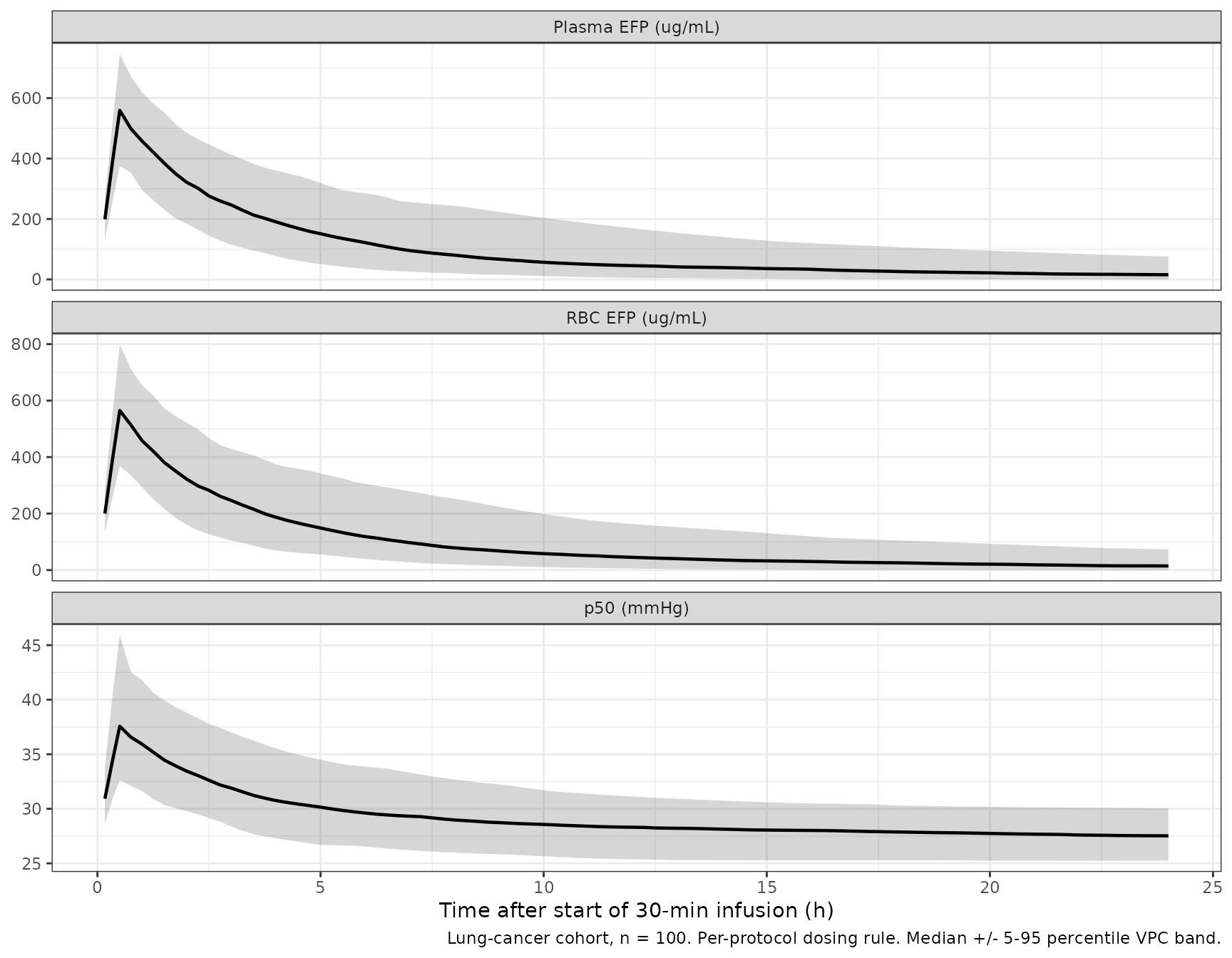
Figure 5 replication - predicted exposure and PD response vs body weight
Figure 5 of Gastonguay 2005 shows the predicted plasma EFP, RBC EFP, and change-from-baseline p50 plotted against body weight for subjects following the per-protocol dosing rule. We replicate this here with the same dosing rule applied to the pooled virtual cohort.
# Read off the per-subject Cmax of plasma, RBC, and change-from-baseline p50
# from the typical-value simulation (matches the paper's "predicted" values).
fig5_summary <- sim_typical |>
  group_by(id, WT, dose_mg, cancer_type) |>
  summarise(
    plasma_cmax = max(Cc,   na.rm = TRUE),
    rbc_cmax    = max(Crbc, na.rm = TRUE),
    dp50_max    = max(p50,  na.rm = TRUE) - 26.9, # change from baseline INTp50
    .groups = "drop"
  ) |>
  filter(is.finite(plasma_cmax))

fig5_long <- fig5_summary |>
  select(id, WT, plasma_cmax, rbc_cmax, dp50_max) |>
  pivot_longer(cols = c(plasma_cmax, rbc_cmax, dp50_max),
               names_to = "metric", values_to = "value") |>
  mutate(panel = factor(
    metric,
    levels = c("plasma_cmax", "rbc_cmax", "dp50_max"),
    labels = c("Predicted plasma EFP Cmax (ug/mL)",
               "Predicted RBC EFP Cmax (ug/mL)",
               "Predicted change in p50 (mmHg)")
  ))

ggplot(fig5_long, aes(WT, value)) +
  geom_point(alpha = 0.45) +
  geom_smooth(method = "loess", se = FALSE, linewidth = 0.8,
              colour = "steelblue", linetype = "dashed") +
  facet_wrap(~panel, scales = "free_y", ncol = 3) +
  labs(x = "Body weight (kg)", y = NULL,
       caption = "Replicates Figure 5 of Gastonguay 2005: per-protocol dosing rule applied to a virtual cohort.") +
  theme_bw()
#> `geom_smooth()` using formula = 'y ~ x'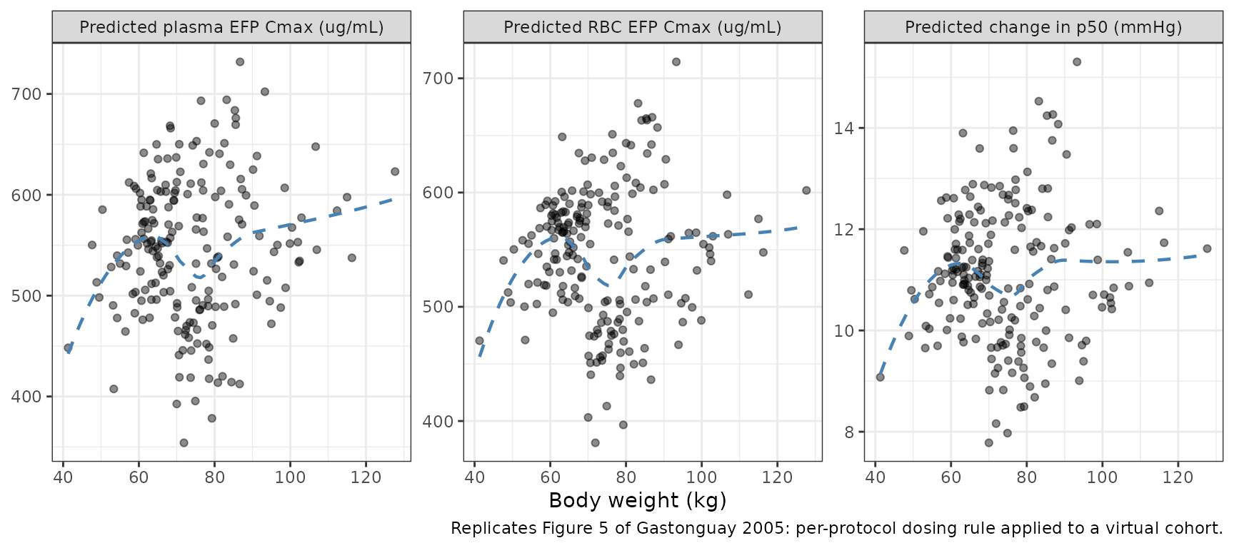
PKNCA validation
NCA of the plasma EFP profile after the single 30-minute infusion. The paper does not report explicit NCA values; the check here is a self-consistency check that the typical-value NCA agrees with hand-computable expectations from the structural model (typical CL = 1.88 L/h, V1 = 10.5 L for the reference covariate combination so the apparent V_ss = V1 + V2 ~ 28.6 L and the terminal half-life is on the order of ln(2) * V_ss / CL ~ 10.5 h).
# Use the typical-value simulation; this is a deterministic NCA crosscheck
# against the published typical-value parameters.
sim_nca <- sim_typical |>
  filter(!is.na(Cc)) |>
  select(id, time, Cc, cancer_type)

# Guarantee a time = 0 row per (id, cancer_type) so AUC0-* starts at the
# pre-infusion baseline.
sim_nca <- bind_rows(
  sim_nca,
  sim_nca |> distinct(id, cancer_type) |>
    mutate(time = 0, Cc = 0)
) |>
  distinct(id, cancer_type, time, .keep_all = TRUE) |>
  arrange(id, cancer_type, time)

conc_obj <- PKNCA::PKNCAconc(
  sim_nca, Cc ~ time | cancer_type + id,
  concu = "ug/mL", timeu = "h"
)

dose_df <- events |>
  filter(evid == 1) |>
  select(id, time, amt, cancer_type) |>
  mutate(amt = as.numeric(amt))

dose_obj <- PKNCA::PKNCAdose(
  dose_df, amt ~ time | cancer_type + id, doseu = "mg"
)

intervals <- data.frame(
  start       = 0,
  end         = Inf,
  cmax        = TRUE,
  tmax        = TRUE,
  aucinf.obs  = TRUE,
  half.life   = TRUE
)

nca_res <- PKNCA::pk.nca(
  PKNCA::PKNCAdata(conc_obj, dose_obj, intervals = intervals)
)

nca_summary <- as.data.frame(nca_res$result) |>
  filter(PPTESTCD %in% c("cmax", "tmax", "aucinf.obs", "half.life")) |>
  group_by(cancer_type, PPTESTCD) |>
  summarise(median_value = median(PPORRES, na.rm = TRUE),
            .groups = "drop") |>
  tidyr::pivot_wider(names_from = PPTESTCD, values_from = median_value) |>
  dplyr::rename(
    "Cancer-type cohort" = cancer_type,
    "Cmax (ug/mL)"       = cmax,
    "Tmax (h)"           = tmax,
    "AUCinf,obs (ug*h/mL)" = aucinf.obs,
    "Half-life (h)"      = half.life
  )

knitr::kable(
  nca_summary,
  digits  = c(0, 1, 2, 0, 1),
  caption = "Median NCA values per cancer-type cohort from the typical-value simulation. The per-protocol dosing rule produces different per-subject doses by sex/weight; the cancer-type effects only modify SLPp50 (not PK) so the plasma NCA values are essentially equal across the two cohorts and depend on the dose distribution only."
)| Cancer-type cohort | AUCinf,obs (ug*h/mL) | Cmax (ug/mL) | Half-life (h) | Tmax (h) |
|---|---|---|---|---|
| breast | 3337.5 | 550.94 | 13 | 0.5 |
| lung | 3407.8 | 547.36 | 13 | 0.5 |
Assumptions and deviations
- Cohort covariate distributions were sampled to approximate the published Table 1 marginal distributions; the original individual covariate values are not public. Specifically, weight (lognormal centered on the median 72.3 kg with SD log(0.18) truncated to [38.6, 129]), height (normal centered on median 169 cm with SD 9.5 truncated to [135, 193]), BSA (computed from weight and height via the Du Bois formula then truncated to [1.31, 2.50]), age (normal centered on median 57 with SD 12 truncated to [28, 87]), albumin (normal centered on 3.6 g/dL with SD 0.5 truncated to [2.2, 5.0]) and a 50/50 sex split.
-
Per-protocol dosing rule from Figure 5 caption (100
mg/kg for males <= 95 kg and females <= 70 kg; 75 mg/kg otherwise)
is applied to assign each virtual subject’s single 30-minute IV
infusion.
DOSE_EFP_MAX_MGis set to this same per-subject value (single-dose simulation). - Cancer-type cohorts. Only lung (reference, n = 100) and breast (CATP = 2, n = 100) are simulated; the cranial-GBM (TUMTP_GLIO) and “other” (TUMTP_OTHER) cancer-type indicators are exercised by the categorical power-model effect on SLPp50 in the model itself but are not enumerated separately in this vignette to keep the cohort under the 200-per-arm cap.
-
Categorical PD multipliers encoded on the log
scale. The paper’s Equation 1 writes the SLPp50 cancer-type
multipliers in product-of-powers form (theta * theta_CATP2^CATP2 *
theta_CATP3^CATP3 * theta_CATP4^CATP4). In the packaged model the
equivalent log-additive form (log(theta) + CATP2 * log(theta_CATP2) + …)
is used so the canonical e_
_ covariate- effect parameters carry log multipliers ( e_breast_slope_p50 = log(1.11),e_glio_slope_p50 = log(1.28),e_other_slope_p50 = log(0.854)). Numerically identical to the paper’s form. - Equation 1 typesetting. Equation 1 does not survive plain-text extraction of the poster PDF; it was recovered by re-extracting it from the PDF via pdftotext, and the explicit reference values used are BSA = 1.8 m^2, AGE = 60 yr, BALB = 3.5 g/dL, MDOS = 6800 mg (all taken directly from the Equation 1 denominators on page 13 of the poster).
-
Baseline albumin units. The paper uses BALB in g/dL
with reference value 3.5 g/dL in Equation 1, while the canonical ALB
covariate is in g/L (SI). The model file converts inline via
alb_gdL <- ALB * 0.1before the power-of-(BALB/3.5) terms; the virtual cohort populates ALB in g/L. -
DOSE_EFP_MAX_MGis a per-subject scalar. The paper’s MDOS covariate is the maximum single-administration dose the subject received, used as a static power-model effect on SLPRBC. In a single-dose simulation this equals the dose itself; in a multi-dose study the column would be the highest assigned single dose across the trial. - Cancer-type composition pooled. The paper’s CATP = 4 (“other”) group pools cancer types other than lung, breast, and cranial GBM (Data section). No further sub-stratification is available; the vignette uses the lung and breast cohorts only as a representative validation.
- PKNCA validation is self-consistency only. The poster does not publish NCA values; the NCA table shows the median Cmax / Tmax / AUC / half-life computed from the deterministic typical-value simulation as a hand-checkable reference (V_ss ~= V1 + V2 = 28.6 L; CL = 1.88 L/h; expected terminal half-life ~ ln(2) * V_ss / CL ~ 10.5 h).