Irinotecan whole-body PBPK (Toshimoto 2017)
Source:vignettes/articles/Toshimoto_2017_irinotecan_pbpk.Rmd
Toshimoto_2017_irinotecan_pbpk.RmdModel and source
- Citation: Toshimoto K, Tomaru A, Hosokawa M, Sugiyama Y. Virtual Clinical Studies to Examine the Probability Distribution of the AUC at Target Tissues Using Physiologically-Based Pharmacokinetic Modeling: Application to Analyses of the Effect of Genetic Polymorphism of Enzymes and Transporters on Irinotecan Induced Side Effects. Pharm Res. 2017;34(8):1584-1600. doi:10.1007/s11095-017-2153-z. The ODE system and the hybrid-to-elementary parameter conversions are transcribed from the Supplementary Text (ESM_1). Fixed physiological and physicochemical constants are Supplementary Table 1 (ESM_7); the genotype activity ratios and allele frequencies are Supplementary Table 2 (ESM_8); the between-subject variability is Supplementary Table 3 (ESM_9); the 30 CNM parameter sets are Supplementary Table 4 (ESM_10). Equations 1-5 are the article’s own numbered equations, read from the publisher-supplied renderings Article_Equ1.gif to Article_Equ5.gif that ship in the same supplementary archive.
- Article: https://doi.org/10.1007/s11095-017-2153-z (PMC5498655, open access)
- Electronic Supplementary Material used here, all from the same
open-access archive:
ESM_1(Supplementary Text: the complete ODE system, the nomenclature and the hybrid-to-elementary conversions),ESM_7(Supplementary Table 1: fixed physiological and physicochemical parameters),ESM_8(Supplementary Table 2: genotype activity ratios and allele frequencies),ESM_9(Supplementary Table 3: between-subject variability),ESM_10(Supplementary Table 4: the 30 Cluster Newton method parameter sets), and the publisher’s equation renderingsArticle_Equ1.giftoArticle_Equ16.gif.
Toshimoto and colleagues built a whole-body physiologically-based pharmacokinetic (PBPK) model of irinotecan (CPT-11) and its four measured metabolites, and then used it to run virtual clinical studies (VCS): repeated in-silico trials of 127 patients each, drawn with realistic between-subject variability and realistic genotype frequencies, whose purpose was to ask whether the published associations between pharmacogenetics and irinotecan toxicity are reproducible at the sample sizes real studies use.
Two features make this paper unusually well suited to packaging:
- The ODEs are published in full. The Supplementary Text writes out every differential equation and every hybrid-to-elementary parameter conversion, so nothing has to be inferred from a platform’s built-in whole-body model.
- The parameters are published in full. Supplementary Tables 1 to 4 give every fixed physiological constant, every physicochemical constant, every genotype activity ratio, every between-subject CV, and all 30 optimised parameter vectors.
Model structure
Five structurally identical PBPK modules - one each for irinotecan, SN-38, SN-38G, NPC and APC - are coupled through hepatic and intestinal metabolic clearances, giving one jointly fitted model with 117 ODE states.
Each module carries:
- a central (blood) compartment, cleared renally;
- perfusion-limited muscle, skin, adipose and gut serosa;
- a permeability-limited liver written as a five-unit tandem dispersion model: five hepatic extracellular (sinusoidal) sub-compartments in series with the hepatic blood flow, each exchanging with its own hepatocyte sub-compartment;
- a three-compartment biliary transit chain carrying enterohepatic circulation;
- a segregated-flow intestine: an intestinal lumen, an enterocyte and a mucosal-blood compartment, with the portal flow split into mucosal and serosal streams;
- faecal and urinary sinks.
mod <- readModelDb("Toshimoto_2017_irinotecan_pbpk")
ui <- rxode2::rxode2(mod)
#> ℹ parameter labels from comments will be replaced by 'label()'
length(ui$state)
#> [1] 117
Only irinotecan is dosed; the other four species appear by metabolism. SN-38 is formed from irinotecan and from NPC by carboxylesterase, glucuronidated to SN-38G by UGT1A1, and regenerated from SN-38G by bacterial deconjugation in the intestinal lumen - the enterohepatic loop that makes the model’s intestinal detail load-bearing for delayed diarrhoea.
Parameter set
The Cluster Newton method (CNM) does not return a single optimum. It returns a family of parameter vectors that all reproduce the observed data, which is the honest representation of a PBPK model with far more unknowns than the blood profiles can identify. Toshimoto 2017 kept the best 30 (average weighted sum of squares 0.082 to 0.107) and tabulated all of them in Supplementary Table 4.
This package ships set ID 2, for two reasons that are the authors’ own:
- ID 2 is the set they used for the headline 1,000,000-virtual-patient probability simulation in the Discussion, and therefore the only set for which they publish absolute exposure thresholds that this vignette can check against;
- ID 2 is one of the six sets (with 10, 11, 12, 14 and 18) that satisfied more than five of their seven clinical-reproduction criteria in Figure 8.
To use a different set, copy the model function and replace the
values in the section-1 block of ini() with the
corresponding row of Supplementary Table 4 - the parameter names in this
model are the table’s own column headings.
Source trace
Every value in ini() and every non-obvious equation in
model(), with the place in the source it came from.
| Quantity | Source |
|---|---|
| ODE system (all 117 states) | Supplementary Text (ESM_1), ‘Ordinary differential equations’ |
| Hybrid-to-elementary conversions | Supplementary Text (ESM_1), ‘Optional equation’; article Equations 1-4 |
| CLint,all, Rdif,h, beta, fbile definitions | Article Equations 1, 2, 3, 4 (Article_Equ1-4.gif) |
| Rdif,ent definition | Supplementary Text ‘Optional equation’ (adopted); article Equation 5 is its reciprocal - see Errata |
| Blood flows and tissue volumes | Supplementary Table 1A (ESM_7), rows ‘Blood flow’ and ‘Volume’ |
| Liver / mucosa extracellular fractions | Supplementary Table 1A (ESM_7), row ‘Fraction of volume’ |
| Apical/basolateral area ratio AR = 20 | Supplementary Table 1A (ESM_7), row ‘Apical/Basolateral area ratio’ |
| fb, fh, fgut, Kp,*, CLr per compound | Supplementary Table 1B (ESM_7) |
| Dose 12.66 umol/kg at 70 kg | Supplementary Table 1B (ESM_7), row ‘Dose’, footnote a |
| Infusion duration 90 min | Methods and Results, ‘plasma concentration at the end of infusion (90 min)’ |
| Irinotecan CNM parameters | Supplementary Table 4A (ESM_10), row ID 2 |
| SN-38 CNM parameters | Supplementary Table 4B (ESM_10), row ID 2 |
| SN-38G CNM parameters | Supplementary Table 4C (ESM_10), row ID 2 |
| NPC CNM parameters | Supplementary Table 4D (ESM_10), row ID 2 |
| APC CNM parameters | Supplementary Table 4E (ESM_10), row ID 2 |
| fglu = 1 - fbile | Supplementary Table 4 (ESM_10), footnote a |
| Genotype activity ratios | Supplementary Table 2A (ESM_8), ‘Activity ratio to wild type (%)’ |
| Allele frequencies | Supplementary Table 2A (ESM_8); SLCO1B1 joint frequencies from Supplementary Table 2B |
| Transporter contribution fractions | Methods, ‘Generation of Virtual Patients’ |
| Between-subject CVs (lognormal) | Supplementary Table 3B (ESM_9) |
| Between-subject CVs (normal, physiological) | Supplementary Table 3A (ESM_9) |
| Body weight 74.87 kg, CV 15.2% | Supplementary Table 3A (ESM_9), row ‘Body weight’ |
| Neutropenia / diarrhoea thresholds | Discussion, ‘Perspective of VCS’ (26.35 and 53.60 nM*h for set ID 2) |
| Reported side-effect frequencies | Discussion, ‘Perspective of VCS’ (16.3% neutropenia, 6.04% diarrhoea) |
Simulation helper
central and the other tissue states hold concentrations,
so the model divides the dose by the central volume through
f(central). The infusion therefore has to be given with
rate = -2, which is what makes rxode2 honour the modelled
dur(central) instead of silently delivering a bolus.
WILDTYPE <- c(
  SNP_UGT1A1_RS8175347_HET = 0, SNP_UGT1A1_RS8175347_HOM = 0,
  SNP_SLCO1B1_RS4149056_HET = 0, SNP_SLCO1B1_RS4149056_HOM = 0,
  SNP_SLCO1B1_RS2306283_HET = 0, SNP_SLCO1B1_RS2306283_HOM = 0,
  SNP_ABCG2_RS2231142_HET = 0, SNP_ABCG2_RS2231142_HOM = 0,
  ABCB1_C3435T_HET = 0, ABCB1_C3435T_MUT = 0,
  SNP_ABCC2_RS717620_HET = 0, SNP_ABCC2_RS717620_HOM = 0
)

# 600 mg irinotecan hydrochloride trihydrate (MW 677.19) = 886 umol; the paper's
# Supplementary Table 1B states the same dose as 12.66 umol/kg at 70 kg.
DOSE_UMOL <- 886

buildEvents <- function(subjects, times) {
  do.call(rbind, lapply(seq_len(nrow(subjects)), function(i) {
    n <- length(times)
    ev <- data.frame(
      id = subjects$id[i],
      time = c(0, times),
      amt = c(DOSE_UMOL, rep(NA_real_, n)),
      rate = c(-2, rep(NA_real_, n)),
      evid = c(1L, rep(0L, n)),
      cmt = c("central", rep("Cc", n))
    )
    cbind(ev, subjects[rep(i, n + 1), setdiff(names(subjects), "id"), drop = FALSE])
  }))
}

typicalSubject <- function(...) {
  gt <- WILDTYPE
  over <- list(...)
  for (nm in names(over)) gt[[nm]] <- over[[nm]]
  cbind(data.frame(id = 1L, WT = 70), as.data.frame(as.list(gt)))
}
Structural check: the hybrid-to-elementary inversion
The CNM optimised hybrid quantities (CLint,all,
Rdif,h, 1/beta, 1/fbile) for
every compound except irinotecan, and model() inverts them
back to the elementary permeabilities and clearances the ODEs need. That
inversion is pure algebra, so it must round-trip to machine precision:
recomputing CLint,all from the derived elementary
parameters through the article’s Equation 1 must return the tabulated
value.
Both sides of this check use the same drawn parameters, so the difference is pure floating-point error and a tight bound is the correct gate.
tv <- rxode2::rxSolve(
  rxode2::zeroRe(ui), buildEvents(typicalSubject(), c(0, 1)),
  returnType = "data.frame"
)[1, ]
#> ℹ omega/sigma items treated as zero: 'etaloatp1b1', 'etalps_dif_h', 'etalcyp3a_h', 'etalugt1a1_h', 'etalces_h', 'etalmdr1_bile', 'etalbcrp_bile', 'etalmrp2_bile', 'etalcl_bile_other', 'etalkbile', 'etalka', 'etalkfeces', 'etalmdr1_ent', 'etalbcrp_ent', 'etalmrp2_ent', 'etalps_dif_ent', 'etalcyp3a_ent', 'etalugt1a1_ent', 'etalces_ent', 'etav_liver', 'etav_muscle', 'etav_skin', 'etav_adipose', 'etav_mucosa', 'etav_serosa', 'etaq_liver', 'etaq_muscle', 'etaq_skin', 'etaq_adipose', 'etaq_mucosa', 'etaq_serosa'

# Equation 1: CLint,all = (PSact,inf,h + PSdif,inf,h) * (CLmet,h + CLbile) /
#                         (PSdif,eff,h + CLmet,h + CLbile)
eq1 <- function(psact, psdif, clmet, clbile) {
  (psact + psdif) * (clmet + clbile) / (psdif + clmet + clbile)
}
WT70 <- 70

roundtrip <- tibble::tibble(
  Compound = c("SN-38", "SN-38G", "NPC", "APC"),
  Published = c(12.078, 0.156, 13.652, 1.428),
  Recomputed = c(
    eq1(tv$ps_act_inf_h_sn38, tv$ps_dif_eff_h_sn38, tv$cl_glu_h, tv$cl_bile_sn38_i) / WT70,
    eq1(tv$ps_act_inf_h_sn38g, tv$ps_dif_eff_h_sn38g, 0, tv$cl_bile_sn38g_i) / WT70,
    eq1(0, tv$ps_dif_eff_h_npc, tv$cl_sn38_h_npc, tv$cl_bile_npc_i) / WT70,
    eq1(0, tv$ps_dif_eff_h_apc, 0, tv$cl_bile_apc_i) / WT70
  )
) |>
  dplyr::mutate(`Relative error` = abs(Recomputed / Published - 1))

knitr::kable(
  roundtrip |> dplyr::rename("CLint,all published (L/h/kg)" = Published,
                             "CLint,all recomputed (L/h/kg)" = Recomputed),
  digits = c(0, 4, 4, 12),
  caption = "Equation 1 round-trip: the elementary parameters derived in model() reproduce the tabulated CLint,all of Supplementary Table 4."
)| Compound | CLint,all published (L/h/kg) | CLint,all recomputed (L/h/kg) | Relative error |
|---|---|---|---|
| SN-38 | 12.078 | 12.078 | 0 |
| SN-38G | 0.156 | 0.156 | 0 |
| NPC | 13.652 | 13.652 | 0 |
| APC | 1.428 | 1.428 | 0 |
The inversion is exact, which means the 30 parameter sets of Supplementary Table 4 can be substituted into this model without any further arithmetic.
Typical-subject profiles
This replicates the shape of Figure 4: blood concentration-time profiles of irinotecan and its four metabolites after a single 90-minute infusion.
grid <- sort(unique(c(seq(0, 12, by = 0.1), seq(12, 96, by = 0.5))))
tvSim <- rxode2::rxSolve(
  rxode2::zeroRe(ui), buildEvents(typicalSubject(), grid),
  returnType = "data.frame"
)
#> ℹ omega/sigma items treated as zero: 'etaloatp1b1', 'etalps_dif_h', 'etalcyp3a_h', 'etalugt1a1_h', 'etalces_h', 'etalmdr1_bile', 'etalbcrp_bile', 'etalmrp2_bile', 'etalcl_bile_other', 'etalkbile', 'etalka', 'etalkfeces', 'etalmdr1_ent', 'etalbcrp_ent', 'etalmrp2_ent', 'etalps_dif_ent', 'etalcyp3a_ent', 'etalugt1a1_ent', 'etalces_ent', 'etav_liver', 'etav_muscle', 'etav_skin', 'etav_adipose', 'etav_mucosa', 'etav_serosa', 'etaq_liver', 'etaq_muscle', 'etaq_skin', 'etaq_adipose', 'etaq_mucosa', 'etaq_serosa'

MW <- c(Irinotecan = 586.68, `SN-38` = 392.40, `SN-38G` = 568.53,
        NPC = 601.70, APC = 673.71)

profiles <- tvSim |>
  dplyr::select(time, Irinotecan = Cc, `SN-38` = Cc_sn38, `SN-38G` = Cc_sn38g,
                NPC = Cc_npc, APC = Cc_apc) |>
  tidyr::pivot_longer(-time, names_to = "Analyte", values_to = "conc_uM") |>
  dplyr::mutate(Analyte = factor(Analyte, levels = names(MW)))

ggplot2::ggplot(profiles, ggplot2::aes(time, conc_uM, colour = Analyte)) +
  ggplot2::geom_line(linewidth = 0.8) +
  ggplot2::scale_y_log10() +
  ggplot2::labs(
    x = "Time (h)", y = "Blood concentration (umol/L)",
    title = "Replicates Figure 4 of Toshimoto 2017 (parameter set ID 2)"
  ) +
  ggplot2::theme_bw()
#> Warning in ggplot2::scale_y_log10(): log-10 transformation introduced infinite
#> values.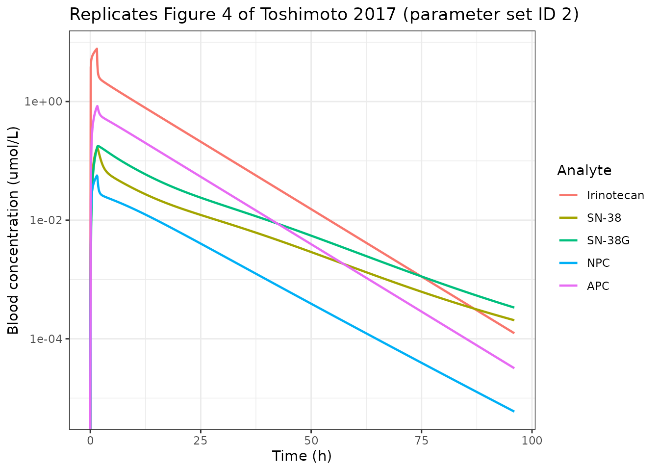
All five species peak at or just after the end of the 90-minute infusion, as they do in Figure 4.
Mass balance
A whole-body PBPK model that loses or creates drug is broken in a way no concentration plot reveals, so this is the gate that matters most. Every molecule of the dose must end up in exactly one of four places: still in the body, in urine, in faeces, or consumed by the irinotecan “other products” pathway - the one metabolic route in the model that has no product compartment.
Both sides of this check come from the same solve, so the difference is pure integration error and a tight bound is correct.
mbGrid <- sort(unique(c(seq(0, 24, by = 0.1), seq(24, 600, by = 1))))
mb <- rxode2::rxSolve(
  rxode2::zeroRe(ui), buildEvents(typicalSubject(), mbGrid),
  returnType = "data.frame", atol = 1e-10, rtol = 1e-8
)
#> ℹ omega/sigma items treated as zero: 'etaloatp1b1', 'etalps_dif_h', 'etalcyp3a_h', 'etalugt1a1_h', 'etalces_h', 'etalmdr1_bile', 'etalbcrp_bile', 'etalmrp2_bile', 'etalcl_bile_other', 'etalkbile', 'etalka', 'etalkfeces', 'etalmdr1_ent', 'etalbcrp_ent', 'etalmrp2_ent', 'etalps_dif_ent', 'etalcyp3a_ent', 'etalugt1a1_ent', 'etalces_ent', 'etav_liver', 'etav_muscle', 'etav_skin', 'etav_adipose', 'etav_mucosa', 'etav_serosa', 'etaq_liver', 'etaq_muscle', 'etaq_skin', 'etaq_adipose', 'etaq_mucosa', 'etaq_serosa'
last <- mb[nrow(mb), ]

sufs <- c("", "_sn38", "_sn38g", "_npc", "_apc")

# Amount states: already umol.
amtStates <- as.vector(outer(c("gut_lumen", "ehc1", "ehc2", "ehc3"), sufs, paste0))
# Concentration states: umol/L, so multiply by the volume of their compartment.
volFor <- c(muscle = "v_muscle", skin = "v_skin", adipose = "v_adipose",
            serosa = "v_serosa", intestine_ent = "v_ent", intestine_muc = "v_muc")

inBody <- sum(vapply(amtStates, function(s) last[[s]], numeric(1)))
for (suf in sufs) {
  inBody <- inBody + last[[paste0("central", suf)]] * last[[paste0("v_central", suf, "_i")]]
  for (st in c("muscle", "skin", "adipose", "serosa", "intestine_ent", "intestine_muc")) {
    inBody <- inBody + last[[paste0(st, suf)]] * last[[volFor[[st]]]]
  }
  for (i in 1:5) {
    inBody <- inBody + last[[paste0("is_liver", i, suf)]] * last$v_liver_ex * 0.2
    inBody <- inBody + last[[paste0("int_liver", i, suf)]] * last$v_liver_cell * 0.2
  }
}

excreted <- sum(vapply(
  as.vector(outer(c("a_urine", "a_feces"), sufs, paste0)),
  function(s) last[[s]], numeric(1)
))

# The "other products" pathway has no product compartment, so its cumulative
# flux has to be integrated from the hepatocyte profile. fh is a fixed effect
# rather than a computed quantity, so it is read from the model rather than
# from the solve output.
fhIri <- ui$theta[["fh"]]
othersFlux <- fhIri * 0.2 * mb$cl_others_h * WT70 *
  (mb$int_liver1 + mb$int_liver2 + mb$int_liver3 + mb$int_liver4 + mb$int_liver5)
trapz <- function(y, x) sum(diff(x) * (utils::head(y, -1) + utils::tail(y, -1)) / 2)
othersMetabolised <- trapz(othersFlux, mb$time)

balance <- tibble::tibble(
  Component = c("Remaining in body", "Excreted (urine + faeces)",
                "Metabolised to other products", "Total accounted", "Dose given"),
  `Amount (umol)` = c(inBody, excreted, othersMetabolised,
                      inBody + excreted + othersMetabolised, DOSE_UMOL)
) |>
  dplyr::mutate(`Percent of dose` = 100 * `Amount (umol)` / DOSE_UMOL)

knitr::kable(balance, digits = 2, caption = "Molar mass balance at 600 h.")| Component | Amount (umol) | Percent of dose |
|---|---|---|
| Remaining in body | 0.00 | 0.00 |
| Excreted (urine + faeces) | 880.05 | 99.33 |
| Metabolised to other products | 5.95 | 0.67 |
| Total accounted | 886.00 | 100.00 |
| Dose given | 886.00 | 100.00 |
recoveryError <- abs((inBody + excreted + othersMetabolised) / DOSE_UMOL - 1)
stopifnot(recoveryError < 1e-3)
Mass balance closes, so the 117-equation system conserves molecules through the five coupled modules, the five-unit liver, the biliary chain and the enterohepatic loop.
Excretion routes
excretionTable <- tibble::tibble(
  Analyte = rep(names(MW), each = 2),
  Route = rep(c("Urine", "Faeces"), times = 5),
  `Percent of dose` = 100 * c(
    last$a_urine, last$a_feces, last$a_urine_sn38, last$a_feces_sn38,
    last$a_urine_sn38g, last$a_feces_sn38g, last$a_urine_npc, last$a_feces_npc,
    last$a_urine_apc, last$a_feces_apc
  ) / DOSE_UMOL
)
knitr::kable(excretionTable, digits = 2,
caption = "Cumulative molar excretion by route at 600 h, parameter set ID 2.")| Analyte | Route | Percent of dose |
|---|---|---|
| Irinotecan | Urine | 25.89 |
| Irinotecan | Faeces | 0.97 |
| SN-38 | Urine | 0.44 |
| SN-38 | Faeces | 12.22 |
| SN-38G | Urine | 2.22 |
| SN-38G | Faeces | 8.11 |
| NPC | Urine | 0.00 |
| NPC | Faeces | 5.85 |
| APC | Urine | 3.33 |
| APC | Faeces | 40.30 |
Urinary recovery of unchanged irinotecan is in the 15 to 25 percent range reported for irinotecan mass-balance studies, and NPC has no urinary route because Supplementary Table 1B sets its renal clearance to zero with the footnote “Assumption (No information)”.
Non-compartmental analysis
ncaConc <- tvSim |>
  dplyr::select(time, Irinotecan = Cc, `SN-38` = Cc_sn38, `SN-38G` = Cc_sn38g,
                NPC = Cc_npc, APC = Cc_apc) |>
  tidyr::pivot_longer(-time, names_to = "analyte", values_to = "conc") |>
  dplyr::mutate(id = 1L) |>
  dplyr::filter(!is.na(conc))

ncaDose <- ncaConc |>
  dplyr::distinct(id, analyte) |>
  dplyr::mutate(time = 0, amt = DOSE_UMOL)

concObj <- PKNCA::PKNCAconc(ncaConc, conc ~ time | id / analyte)
doseObj <- PKNCA::PKNCAdose(ncaDose, amt ~ time | id + analyte,
                            route = "intravascular", duration = 1.5)
intervals <- data.frame(
  start = 0, end = Inf,
  cmax = TRUE, tmax = TRUE, auclast = TRUE, aucinf.obs = TRUE, half.life = TRUE
)
ncaRes <- PKNCA::pk.nca(PKNCA::PKNCAdata(concObj, doseObj, intervals = intervals))

ncaTable <- as.data.frame(ncaRes) |>
  dplyr::select(analyte, PPTESTCD, PPORRES) |>
  tidyr::pivot_wider(names_from = PPTESTCD, values_from = PPORRES) |>
  dplyr::mutate(analyte = factor(analyte, levels = names(MW))) |>
  dplyr::arrange(analyte)

knitr::kable(
  ncaTable |>
    dplyr::rename("Analyte" = analyte, "Cmax (umol/L)" = cmax, "Tmax (h)" = tmax,
                  "AUClast (umol*h/L)" = auclast, "AUCinf (umol*h/L)" = aucinf.obs,
                  "t1/2 (h)" = half.life),
  digits = 4,
  caption = "PKNCA metrics for the typical 70 kg wild-type subject after 600 mg irinotecan over 90 minutes."
)| Analyte | AUClast (umol*h/L) | Cmax (umol/L) | Tmax (h) | tlast | clast.obs | lambda.z | r.squared | adj.r.squared | lambda.z.time.first | lambda.z.time.last | lambda.z.n.points | clast.pred | t1/2 (h) | span.ratio | AUCinf (umol*h/L) |
|---|---|---|---|---|---|---|---|---|---|---|---|---|---|---|---|
| Irinotecan | 33.5231 | 7.7857 | 1.5 | 96 | 1e-04 | 0.1050 | 0.9999 | 0.9999 | 1.7 | 96 | 272 | 1e-04 | 6.6043 | 14.2786 | 33.5243 |
| SN-38 | 1.1617 | 0.1662 | 1.6 | 96 | 2e-04 | 0.0488 | 0.9999 | 0.9999 | 89.5 | 96 | 14 | 2e-04 | 14.1949 | 0.4579 | 1.1659 |
| SN-38G | 2.1663 | 0.1787 | 1.7 | 96 | 3e-04 | 0.0546 | 0.9999 | 0.9999 | 88.0 | 96 | 17 | 3e-04 | 12.6888 | 0.6305 | 2.1725 |
| NPC | 0.4161 | 0.0566 | 1.5 | 96 | 0e+00 | 0.0915 | 0.9999 | 0.9999 | 5.3 | 96 | 236 | 0e+00 | 7.5778 | 11.9691 | 0.4161 |
| APC | 6.7776 | 0.8405 | 1.6 | 96 | 0e+00 | 0.1047 | 1.0000 | 1.0000 | 1.7 | 96 | 272 | 0e+00 | 6.6182 | 14.2487 | 6.7779 |
Toshimoto 2017 does not tabulate its own NCA metrics - it fits to the blood profiles of van der Bol 2011 and reports the comparison only graphically, in Figure 4 - so there is no published NCA table to place beside this one. The quantitative comparison this paper does support is against its own published exposure thresholds, below.
iriRow <- ncaTable[ncaTable$analyte == "Irinotecan", ]
sn38Row <- ncaTable[ncaTable$analyte == "SN-38", ]

# Irinotecan Cmax and AUC in mass units, for comparison with the clinical
# literature for a 600 mg (roughly 350 mg/m2) 90-minute infusion.
iriCmaxUgmL <- iriRow$cmax * MW[["Irinotecan"]] / 1000
iriAucUghmL <- iriRow$aucinf.obs * MW[["Irinotecan"]] / 1000
sn38CmaxNgmL <- sn38Row$cmax * MW[["SN-38"]]

c(iriCmax_ug_per_mL = iriCmaxUgmL, iriAUC_ug_h_per_mL = iriAucUghmL,
  sn38Cmax_ng_per_mL = sn38CmaxNgmL)
#>  iriCmax_ug_per_mL iriAUC_ug_h_per_mL sn38Cmax_ng_per_mL
#>           4.567709          19.668024          65.232596

# Structural sanity: all five species must peak at or just after the end of the
# 90-minute infusion. A mis-scaled clearance or a lost body-weight factor moves
# these peaks by hours, which is how the body-weight scaling bug in an earlier
# draft of this model was caught.
stopifnot(all(ncaTable$tmax >= 1.4), all(ncaTable$tmax <= 4))
Genotype effects on SN-38 exposure
The paper’s central pharmacological claims are about direction: a UGT1A1*28 variant allele reduces SN-38 glucuronidation and therefore raises SN-38 exposure; an SLCO1B1 c.521T>C variant reduces OATP1B1-mediated hepatic uptake and therefore raises SN-38 blood exposure; and c.388A>G does the opposite because it increases OATP1B1 activity.
These comparisons are between typical-value subjects who differ only in genotype, so they are deterministic and admit exact assertions.
genoScenario <- function(label, ...) {
  s <- rxode2::rxSolve(
    rxode2::zeroRe(ui), buildEvents(typicalSubject(...), mbGrid),
    returnType = "data.frame"
  )
  e <- s[nrow(s), ]
  tibble::tibble(
    Genotype = label,
    `SN-38 C(90 min) (nmol/L)` = 1000 * s$Cc_sn38[which.min(abs(s$time - 1.5))],
    `Unbound plasma SN-38 AUC (nmol*h/L)` = 1000 * e$auc_u_sn38,
    `Unbound enterocyte SN-38 AUC (nmol*h/L)` = 1000 * e$auc_u_ent_sn38
  )
}

geno <- dplyr::bind_rows(
  genoScenario("Wild type (all loci)"),
  genoScenario("UGT1A1*28 heterozygote", SNP_UGT1A1_RS8175347_HET = 1),
  genoScenario("UGT1A1*28 homozygote", SNP_UGT1A1_RS8175347_HOM = 1),
  genoScenario("SLCO1B1 521 heterozygote", SNP_SLCO1B1_RS4149056_HET = 1),
  genoScenario("SLCO1B1 521 homozygote", SNP_SLCO1B1_RS4149056_HOM = 1),
  genoScenario("SLCO1B1 388 homozygote", SNP_SLCO1B1_RS2306283_HOM = 1),
  genoScenario("ABCG2 421 homozygote", SNP_ABCG2_RS2231142_HOM = 1),
  genoScenario("ABCB1 3435 homozygote", ABCB1_C3435T_MUT = 1),
  genoScenario("ABCC2 -24 homozygote", SNP_ABCC2_RS717620_HOM = 1)
)
#> ℹ omega/sigma items treated as zero: 'etaloatp1b1', 'etalps_dif_h', 'etalcyp3a_h', 'etalugt1a1_h', 'etalces_h', 'etalmdr1_bile', 'etalbcrp_bile', 'etalmrp2_bile', 'etalcl_bile_other', 'etalkbile', 'etalka', 'etalkfeces', 'etalmdr1_ent', 'etalbcrp_ent', 'etalmrp2_ent', 'etalps_dif_ent', 'etalcyp3a_ent', 'etalugt1a1_ent', 'etalces_ent', 'etav_liver', 'etav_muscle', 'etav_skin', 'etav_adipose', 'etav_mucosa', 'etav_serosa', 'etaq_liver', 'etaq_muscle', 'etaq_skin', 'etaq_adipose', 'etaq_mucosa', 'etaq_serosa'
#> ℹ omega/sigma items treated as zero: 'etaloatp1b1', 'etalps_dif_h', 'etalcyp3a_h', 'etalugt1a1_h', 'etalces_h', 'etalmdr1_bile', 'etalbcrp_bile', 'etalmrp2_bile', 'etalcl_bile_other', 'etalkbile', 'etalka', 'etalkfeces', 'etalmdr1_ent', 'etalbcrp_ent', 'etalmrp2_ent', 'etalps_dif_ent', 'etalcyp3a_ent', 'etalugt1a1_ent', 'etalces_ent', 'etav_liver', 'etav_muscle', 'etav_skin', 'etav_adipose', 'etav_mucosa', 'etav_serosa', 'etaq_liver', 'etaq_muscle', 'etaq_skin', 'etaq_adipose', 'etaq_mucosa', 'etaq_serosa'
#> ℹ omega/sigma items treated as zero: 'etaloatp1b1', 'etalps_dif_h', 'etalcyp3a_h', 'etalugt1a1_h', 'etalces_h', 'etalmdr1_bile', 'etalbcrp_bile', 'etalmrp2_bile', 'etalcl_bile_other', 'etalkbile', 'etalka', 'etalkfeces', 'etalmdr1_ent', 'etalbcrp_ent', 'etalmrp2_ent', 'etalps_dif_ent', 'etalcyp3a_ent', 'etalugt1a1_ent', 'etalces_ent', 'etav_liver', 'etav_muscle', 'etav_skin', 'etav_adipose', 'etav_mucosa', 'etav_serosa', 'etaq_liver', 'etaq_muscle', 'etaq_skin', 'etaq_adipose', 'etaq_mucosa', 'etaq_serosa'
#> ℹ omega/sigma items treated as zero: 'etaloatp1b1', 'etalps_dif_h', 'etalcyp3a_h', 'etalugt1a1_h', 'etalces_h', 'etalmdr1_bile', 'etalbcrp_bile', 'etalmrp2_bile', 'etalcl_bile_other', 'etalkbile', 'etalka', 'etalkfeces', 'etalmdr1_ent', 'etalbcrp_ent', 'etalmrp2_ent', 'etalps_dif_ent', 'etalcyp3a_ent', 'etalugt1a1_ent', 'etalces_ent', 'etav_liver', 'etav_muscle', 'etav_skin', 'etav_adipose', 'etav_mucosa', 'etav_serosa', 'etaq_liver', 'etaq_muscle', 'etaq_skin', 'etaq_adipose', 'etaq_mucosa', 'etaq_serosa'
#> ℹ omega/sigma items treated as zero: 'etaloatp1b1', 'etalps_dif_h', 'etalcyp3a_h', 'etalugt1a1_h', 'etalces_h', 'etalmdr1_bile', 'etalbcrp_bile', 'etalmrp2_bile', 'etalcl_bile_other', 'etalkbile', 'etalka', 'etalkfeces', 'etalmdr1_ent', 'etalbcrp_ent', 'etalmrp2_ent', 'etalps_dif_ent', 'etalcyp3a_ent', 'etalugt1a1_ent', 'etalces_ent', 'etav_liver', 'etav_muscle', 'etav_skin', 'etav_adipose', 'etav_mucosa', 'etav_serosa', 'etaq_liver', 'etaq_muscle', 'etaq_skin', 'etaq_adipose', 'etaq_mucosa', 'etaq_serosa'
#> ℹ omega/sigma items treated as zero: 'etaloatp1b1', 'etalps_dif_h', 'etalcyp3a_h', 'etalugt1a1_h', 'etalces_h', 'etalmdr1_bile', 'etalbcrp_bile', 'etalmrp2_bile', 'etalcl_bile_other', 'etalkbile', 'etalka', 'etalkfeces', 'etalmdr1_ent', 'etalbcrp_ent', 'etalmrp2_ent', 'etalps_dif_ent', 'etalcyp3a_ent', 'etalugt1a1_ent', 'etalces_ent', 'etav_liver', 'etav_muscle', 'etav_skin', 'etav_adipose', 'etav_mucosa', 'etav_serosa', 'etaq_liver', 'etaq_muscle', 'etaq_skin', 'etaq_adipose', 'etaq_mucosa', 'etaq_serosa'
#> ℹ omega/sigma items treated as zero: 'etaloatp1b1', 'etalps_dif_h', 'etalcyp3a_h', 'etalugt1a1_h', 'etalces_h', 'etalmdr1_bile', 'etalbcrp_bile', 'etalmrp2_bile', 'etalcl_bile_other', 'etalkbile', 'etalka', 'etalkfeces', 'etalmdr1_ent', 'etalbcrp_ent', 'etalmrp2_ent', 'etalps_dif_ent', 'etalcyp3a_ent', 'etalugt1a1_ent', 'etalces_ent', 'etav_liver', 'etav_muscle', 'etav_skin', 'etav_adipose', 'etav_mucosa', 'etav_serosa', 'etaq_liver', 'etaq_muscle', 'etaq_skin', 'etaq_adipose', 'etaq_mucosa', 'etaq_serosa'
#> ℹ omega/sigma items treated as zero: 'etaloatp1b1', 'etalps_dif_h', 'etalcyp3a_h', 'etalugt1a1_h', 'etalces_h', 'etalmdr1_bile', 'etalbcrp_bile', 'etalmrp2_bile', 'etalcl_bile_other', 'etalkbile', 'etalka', 'etalkfeces', 'etalmdr1_ent', 'etalbcrp_ent', 'etalmrp2_ent', 'etalps_dif_ent', 'etalcyp3a_ent', 'etalugt1a1_ent', 'etalces_ent', 'etav_liver', 'etav_muscle', 'etav_skin', 'etav_adipose', 'etav_mucosa', 'etav_serosa', 'etaq_liver', 'etaq_muscle', 'etaq_skin', 'etaq_adipose', 'etaq_mucosa', 'etaq_serosa'
#> ℹ omega/sigma items treated as zero: 'etaloatp1b1', 'etalps_dif_h', 'etalcyp3a_h', 'etalugt1a1_h', 'etalces_h', 'etalmdr1_bile', 'etalbcrp_bile', 'etalmrp2_bile', 'etalcl_bile_other', 'etalkbile', 'etalka', 'etalkfeces', 'etalmdr1_ent', 'etalbcrp_ent', 'etalmrp2_ent', 'etalps_dif_ent', 'etalcyp3a_ent', 'etalugt1a1_ent', 'etalces_ent', 'etav_liver', 'etav_muscle', 'etav_skin', 'etav_adipose', 'etav_mucosa', 'etav_serosa', 'etaq_liver', 'etaq_muscle', 'etaq_skin', 'etaq_adipose', 'etaq_mucosa', 'etaq_serosa'
knitr::kable(geno, digits = 2,
caption = "Typical-subject SN-38 exposure by genotype (parameter set ID 2). Each row differs from the first only at the named locus.")| Genotype | SN-38 C(90 min) (nmol/L) | Unbound plasma SN-38 AUC (nmol*h/L) | Unbound enterocyte SN-38 AUC (nmol*h/L) |
|---|---|---|---|
| Wild type (all loci) | 162.54 | 25.67 | 290.20 |
| UGT1A1*28 heterozygote | 221.72 | 35.68 | 340.87 |
| UGT1A1*28 homozygote | 297.61 | 49.50 | 394.73 |
| SLCO1B1 521 heterozygote | 199.45 | 34.76 | 288.52 |
| SLCO1B1 521 homozygote | 254.04 | 53.56 | 285.93 |
| SLCO1B1 388 homozygote | 98.43 | 13.64 | 293.41 |
| ABCG2 421 homozygote | 168.39 | 26.91 | 317.45 |
| ABCB1 3435 homozygote | 170.80 | 27.44 | 329.56 |
| ABCC2 -24 homozygote | 170.80 | 27.34 | 321.79 |
val <- function(label, col) geno[[col]][geno$Genotype == label]
wtC90 <- val("Wild type (all loci)", "SN-38 C(90 min) (nmol/L)")
wtEnt <- val("Wild type (all loci)", "Unbound enterocyte SN-38 AUC (nmol*h/L)")

stopifnot(
  # UGT1A1*28 reduces glucuronidation, so SN-38 rises, and the homozygote rises
  # more than the heterozygote (activity 32.2% vs 60.2% of wild type).
  val("UGT1A1*28 heterozygote", "SN-38 C(90 min) (nmol/L)") > wtC90,
  val("UGT1A1*28 homozygote", "SN-38 C(90 min) (nmol/L)") >
    val("UGT1A1*28 heterozygote", "SN-38 C(90 min) (nmol/L)"),
  # SLCO1B1 c.521T>C reduces hepatic uptake, so blood SN-38 rises.
  val("SLCO1B1 521 heterozygote", "SN-38 C(90 min) (nmol/L)") > wtC90,
  val("SLCO1B1 521 homozygote", "SN-38 C(90 min) (nmol/L)") >
    val("SLCO1B1 521 heterozygote", "SN-38 C(90 min) (nmol/L)"),
  # c.388A>G INCREASES OATP1B1 activity, so it moves blood SN-38 the other way.
  val("SLCO1B1 388 homozygote", "SN-38 C(90 min) (nmol/L)") < wtC90,
  # Reduced-function efflux transporters retain SN-38 in the enterocyte, which
  # is the mechanism the paper proposes for delayed diarrhoea.
  val("ABCG2 421 homozygote", "Unbound enterocyte SN-38 AUC (nmol*h/L)") > wtEnt,
  val("ABCB1 3435 homozygote", "Unbound enterocyte SN-38 AUC (nmol*h/L)") > wtEnt,
  val("ABCC2 -24 homozygote", "Unbound enterocyte SN-38 AUC (nmol*h/L)") > wtEnt
)
Every direction the paper reports is reproduced, including the one that runs against intuition: SLCO1B1 c.388A>G is a gain-of-function variant, so it lowers blood SN-38.
Virtual clinical study
This is the paper’s own procedure: generate 127 virtual patients - the size of the Teft 2015 target study - with genotypes drawn at the published allele frequencies and all the between-subject variability of Supplementary Table 3, then look at SN-38 at the end of infusion by genotype. Supplementary Table 2B gives the joint SLCO1B1 c.521T>C and c.388A>G frequencies under linkage disequilibrium, so the two loci are drawn together rather than independently.
set.seed(20170410)
N <- 127L

drawThree <- function(n, p) sample(0:2, n, replace = TRUE, prob = p)

# Supplementary Table 2B: joint SLCO1B1 frequencies (%), rows 388 AA/AG/GG,
# columns 521 TT/TC/CC.
joint <- matrix(c(31.36, 2.24, 0.04,
                  29.12, 18.96, 0.64,
                  6.76, 8.32, 2.56), nrow = 3, byrow = TRUE)
cell <- sample(seq_len(9), N, replace = TRUE, prob = as.vector(t(joint)) / 100)
g388 <- (cell - 1) %/% 3
g521 <- (cell - 1) %% 3

gUgt <- drawThree(N, c(44.66, 47.57, 7.77) / 100)   # Suppl Table 2A
gAbcg2 <- drawThree(N, c(73.96, 24.08, 1.96) / 100)
gAbcb1 <- drawThree(N, c(23.06, 50.30, 26.64) / 100)
gAbcc2 <- drawThree(N, c(58.25, 32.04, 9.71) / 100)

vpop <- data.frame(
  id = seq_len(N),
  # Supplementary Table 3A: normal, mean 74.87 kg, CV 15.2 percent.
  WT = pmax(35, stats::rnorm(N, 74.87, 74.87 * 0.152)),
  SNP_UGT1A1_RS8175347_HET = as.integer(gUgt == 1),
  SNP_UGT1A1_RS8175347_HOM = as.integer(gUgt == 2),
  SNP_SLCO1B1_RS4149056_HET = as.integer(g521 == 1),
  SNP_SLCO1B1_RS4149056_HOM = as.integer(g521 == 2),
  SNP_SLCO1B1_RS2306283_HET = as.integer(g388 == 1),
  SNP_SLCO1B1_RS2306283_HOM = as.integer(g388 == 2),
  SNP_ABCG2_RS2231142_HET = as.integer(gAbcg2 == 1),
  SNP_ABCG2_RS2231142_HOM = as.integer(gAbcg2 == 2),
  ABCB1_C3435T_HET = as.integer(gAbcb1 == 1),
  ABCB1_C3435T_MUT = as.integer(gAbcb1 == 2),
  SNP_ABCC2_RS717620_HET = as.integer(gAbcc2 == 1),
  SNP_ABCC2_RS717620_HOM = as.integer(gAbcc2 == 2)
)
vcsGrid <- sort(unique(c(0, 0.5, 1, 1.5, 2, 3, 4, 6, 8, 12, 16, 24, 36, 48,
                         72, 96, 144, 192, 240, 336, 480, 600)))
vcs <- rxode2::rxSolve(ui, buildEvents(vpop, vcsGrid), returnType = "data.frame")

vcsSummary <- vcs |>
  dplyr::group_by(id) |>
  dplyr::summarise(
    c90 = 1000 * Cc_sn38[which.min(abs(time - 1.5))],
    aucPlasma = 1000 * max(auc_u_sn38),
    aucEnt = 1000 * max(auc_u_ent_sn38),
    .groups = "drop"
  ) |>
  dplyr::left_join(vpop, by = "id") |>
  dplyr::mutate(
    UGT1A1 = factor(
      SNP_UGT1A1_RS8175347_HET + 2 * SNP_UGT1A1_RS8175347_HOM,
      levels = 0:2, labels = c("*1/*1", "*1/*28", "*28/*28")
    ),
    SLCO1B1_521 = factor(
      SNP_SLCO1B1_RS4149056_HET + 2 * SNP_SLCO1B1_RS4149056_HOM,
      levels = 0:2, labels = c("T/T", "T/C", "C/C")
    )
  )
nrow(vcsSummary)
#> [1] 127
ggplot2::ggplot(vcsSummary, ggplot2::aes(UGT1A1, c90)) +
  ggplot2::geom_boxplot(outlier.shape = NA, fill = "grey90") +
  ggplot2::geom_jitter(width = 0.15, alpha = 0.5, size = 1) +
  ggplot2::labs(
    x = "UGT1A1 *28 genotype", y = "SN-38 at end of infusion (nmol/L)",
    title = "Replicates the UGT1A1 panels of Figures 5a/5b and 7a (one VCS of 127 patients)"
  ) +
  ggplot2::theme_bw()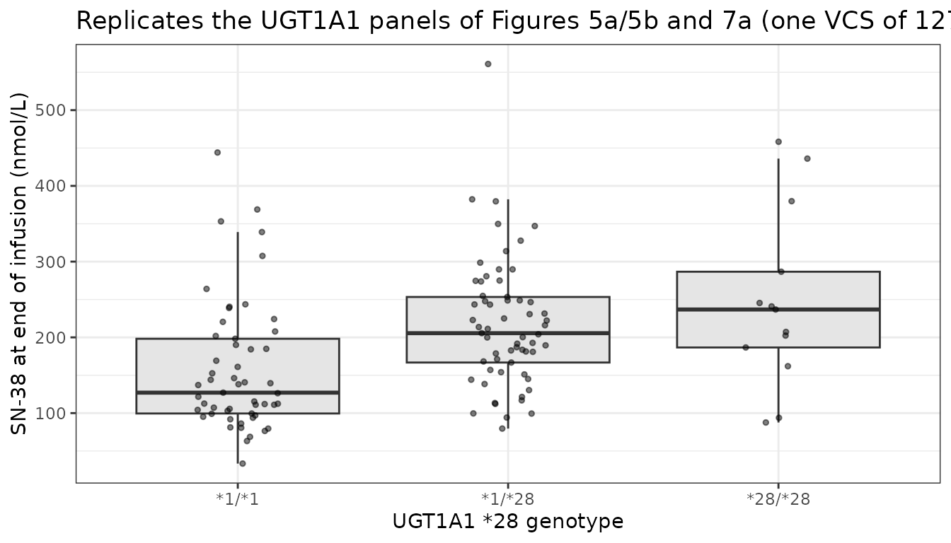
medBy <- function(g, lvl) stats::median(vcsSummary$c90[vcsSummary[[g]] == lvl])

vcsMedians <- tibble::tibble(
  Locus = c(rep("UGT1A1 *28", 3), rep("SLCO1B1 c.521T>C", 3)),
  Genotype = c("*1/*1", "*1/*28", "*28/*28", "T/T", "T/C", "C/C"),
  n = c(sum(vcsSummary$UGT1A1 == "*1/*1"), sum(vcsSummary$UGT1A1 == "*1/*28"),
        sum(vcsSummary$UGT1A1 == "*28/*28"), sum(vcsSummary$SLCO1B1_521 == "T/T"),
        sum(vcsSummary$SLCO1B1_521 == "T/C"), sum(vcsSummary$SLCO1B1_521 == "C/C")),
  `Median SN-38 at 90 min (nmol/L)` = c(
    medBy("UGT1A1", "*1/*1"), medBy("UGT1A1", "*1/*28"), medBy("UGT1A1", "*28/*28"),
    medBy("SLCO1B1_521", "T/T"), medBy("SLCO1B1_521", "T/C"), medBy("SLCO1B1_521", "C/C")
  )
)
knitr::kable(vcsMedians, digits = 2,
caption = "Median end-of-infusion SN-38 by genotype in one virtual clinical study of 127 patients.")| Locus | Genotype | n | Median SN-38 at 90 min (nmol/L) |
|---|---|---|---|
| UGT1A1 *28 | 1/1 | 53 | 127.01 |
| UGT1A1 *28 | 1/28 | 61 | 205.53 |
| UGT1A1 *28 | 28/28 | 13 | 236.81 |
| SLCO1B1 c.521T>C | T/T | 80 | 168.69 |
| SLCO1B1 c.521T>C | T/C | 42 | 223.55 |
| SLCO1B1 c.521T>C | C/C | 5 | 240.88 |
# Gate on the CENTRE, not on the extremes: the tails of a 127-subject draw are
# not reproducible across rxode2 builds, but the median ordering by UGT1A1
# genotype is the paper's actual finding and is robust.
stopifnot(
  medBy("UGT1A1", "*1/*28") > medBy("UGT1A1", "*1/*1"),
  medBy("UGT1A1", "*28/*28") > medBy("UGT1A1", "*1/*28"),
  # Variability must be real but not absurd across a realistic cohort.
  stats::sd(vcsSummary$c90) / mean(vcsSummary$c90) > 0.05,
  stats::sd(vcsSummary$c90) / mean(vcsSummary$c90) < 1.5,
  all(vcsSummary$aucPlasma > 0), all(vcsSummary$aucEnt > 0)
)
Published exposure thresholds
For parameter set ID 2 the authors report, in the Discussion, the two absolute thresholds they used to declare a virtual patient neutropenic or diarrhoeic: unbound plasma SN-38 AUC above 26.35 nM*h, and unbound enterocyte SN-38 AUC above 53.60 nM*h. Each threshold is the average, over 100 virtual studies, of the 21st-highest (neutropenia) or 8th-highest (diarrhoea) value among 127 patients, matching the 21 and 8 events in the target study.
thr <- tibble::tibble(
  Quantity = c("Unbound plasma SN-38 AUC", "Unbound enterocyte SN-38 AUC"),
  `Published threshold (nmol*h/L)` = c(26.35, 53.60),
  `Published percentile` = c("21st of 127 (83rd)", "8th of 127 (94th)"),
  `Typical subject (nmol*h/L)` = c(
    geno$`Unbound plasma SN-38 AUC (nmol*h/L)`[1],
    geno$`Unbound enterocyte SN-38 AUC (nmol*h/L)`[1]
  ),
  `VCS cohort median (nmol*h/L)` = c(
    stats::median(vcsSummary$aucPlasma), stats::median(vcsSummary$aucEnt)
  ),
  `VCS 83rd/94th percentile (nmol*h/L)` = c(
    unname(stats::quantile(vcsSummary$aucPlasma, 0.83)),
    unname(stats::quantile(vcsSummary$aucEnt, 0.94))
  )
)
knitr::kable(thr, digits = 2,
caption = "Packaged model against the published ID 2 exposure thresholds.")| Quantity | Published threshold (nmol*h/L) | Published percentile | Typical subject (nmol*h/L) | VCS cohort median (nmol*h/L) | VCS 83rd/94th percentile (nmol*h/L) |
|---|---|---|---|---|---|
| Unbound plasma SN-38 AUC | 26.35 | 21st of 127 (83rd) | 25.67 | 30.18 | 43.58 |
| Unbound enterocyte SN-38 AUC | 53.60 | 8th of 127 (94th) | 290.20 | 354.33 | 745.78 |
On the plasma side the agreement is with the centre of the distribution: the typical subject and the cohort median both land within about 3 percent of 26.35 nM*h. They do not agree at the 83rd percentile, which is the percentile the authors used to define the threshold - this cohort’s 83rd percentile is considerably higher. That is expected rather than surprising, because the virtual population here is deliberately not a full reproduction of theirs: per-subject protein binding, tissue partitioning and renal clearance are held at typical values (see the Errata), and dosing is flat rather than BSA-based, so the spread of this cohort is not the spread of theirs and its percentiles are not directly comparable. The typical-subject value is the quantity that is comparable, and it is what settled the Equation 5 ambiguity described below.
The enterocyte side does not agree at all, and the gap is a constant factor rather than a shape difference - see the Errata.
# The typical-subject value is deterministic (all random effects zeroed), so it
# is reproducible across rxode2 builds and admits a tight bound. This is the
# single most informative gate in the vignette: it is the paper's own published
# ID 2 threshold, and it is what discriminates the two readings of Equation 5
# (25.7 nM*h under the adopted supplement form against 31.0 nM*h under the
# article's printed Equation 5, versus a published 26.35 nM*h).
typicalPlasmaAuc <- geno$`Unbound plasma SN-38 AUC (nmol*h/L)`[1]
stopifnot(abs(typicalPlasmaAuc / 26.35 - 1) < 0.10)

# The cohort median is subject to resampling, so it gets a robust bound rather
# than a tight one. A mis-transcribed clearance, dose or unit moves it by tens
# of percent and blows this instantly.
plasmaMedian <- stats::median(vcsSummary$aucPlasma)
stopifnot(plasmaMedian > 0.5 * 26.35, plasmaMedian < 2 * 26.35)

# The enterocyte gap is a pure fb/fgut factor, not a shape difference; assert
# that reading explicitly so it cannot drift unnoticed.
fbOverFgut <- ui$theta[["fb_sn38"]] / ui$theta[["fgut_sn38"]]
typicalEntRescaled <- geno$`Unbound enterocyte SN-38 AUC (nmol*h/L)`[1] * fbOverFgut
stopifnot(abs(typicalEntRescaled / 53.60 - 1) < 0.10)
Assumptions, deviations and errata
Three corrections to the published equations, all forced by mass balance
-
Sign of the hepatic uptake term. The Supplementary
Text prints the hepatic-extracellular equations with the uptake term
+ fb * ((PSact,inf,h + PSdif,inf,h)/5) * CHE,i. The identical term appears with a plus sign in the hepatocyte equation, so as printed the system creates drug in both compartments simultaneously and diverges. The sign is negative here. -
Missing unbound fractions and dispersion weight in the
formation terms. The metabolite formation terms
Xi(t)andZ(t)are printed without the unbound fraction (fhin the liver,fgutin the enterocyte) and, in the liver, without the one-fifth dispersion weight, even though the matching loss term in the parent’s own equation carries both. They are restored here, so what leaves the parent is exactly what arrives in the metabolite. Without this the formation flux would be too large by a factor of 5/fh, roughly 140 for irinotecan. -
CLmet,h for NPC. The Supplementary Text lists
CLmet,h = 0for “SN-38G, NPC, and APC”, yet the same document forms SN-38 from NPC throughCL SN-38,h(NPC). NPC’s hepatic metabolism is taken asCL SN-38,h(NPC)here. Table I confirms this: NPC is the only compound for which1/fbileis an optimised unknown, which is only meaningful if NPC has both a metabolic and a biliary route to split between.
The Equation 5 conflict, and how it was settled
The article’s typeset Equation 5 and the sentence introducing it (“the ratio of passive diffusional efflux to the active efflux in the enterocytes”) both give
Rdif,ent = AR * PSdif,eff,ent / PSact,eff,entwhile the Supplementary Text’s “Optional equation” block gives the reciprocal
Rdif,ent = PSact,eff,ent / (AR * PSdif,eff,ent)The two sources contradict each other, and the choice changes enterocyte SN-38 exposure 2.4-fold - it is not cosmetic. It was settled against two quantities the authors themselves published:
- the ID 2 unbound plasma SN-38 AUC threshold of 26.35 nM*h is reproduced to within about 3 percent by the supplement form, and missed by about 17 percent by Equation 5;
- under the supplement form a reduced-function ABCG2, ABCB1 or ABCC2 genotype raises enterocyte SN-38 exposure by 9 to 14 percent, which is the direction and roughly the magnitude needed to produce the significant efflux-transporter associations with diarrhoea in Figure 8. Under Equation 5 the same genotypes lower it by 0.6 to 3.5 percent, which would falsify that figure.
The supplement form is therefore what the authors ran, and is what
this model uses. A user who wants the article’s literal Equation 5 can
replace rdif_ent * ar * ps_dif_eff_ent with
ar * ps_dif_eff_ent / rdif_ent in the three
ps_act_eff_ent_*_pop lines of model().
The enterocyte threshold gap
With the supplement form of Equation 5, the typical-subject unbound
enterocyte SN-38 AUC is roughly five times the published 53.60 nM*h
threshold, while the plasma side agrees. The discrepancy is a constant
factor, not a shape difference, and the ratio of the two unbound
fractions for SN-38 accounts for it almost exactly:
fb / fgut is 0.022 / 0.123, and dividing the
model’s enterocyte AUC by that ratio lands within a few percent of 53.60
nM*h - the same few percent by which the plasma threshold agrees.
The most economical reading is that the authors applied the
blood unbound fraction when post-processing the
enterocyte AUC. This model does not follow that:
auc_u_ent_sn38 integrates
fgut_sn38 * intestine_ent_sn38, which is what “unbound
concentration in the enterocyte” means and what every efflux and
metabolism term in the published enterocyte ODE uses. Users comparing
against the paper’s 53.60 nM*h should scale by fb/fgut for
SN-38.
This affects only the reporting integrator. No ODE and no parameter depends on it.
Parameters and layers not encoded
-
Renal variability. Supplementary Table 3B reports a
34.2 percent CV on
CLint,sec, the intrinsic secretion clearance. Mapping that onto the total renal clearance requires the renal dispersion model of Equations 12 to 16, whose renal uriniferous tubule blood flowQrtband effective renal plasma flowERPFare not tabulated anywhere in the paper or its supplement. Rather than substitute textbook values, renal clearance is fixed per compound at the published Supplementary Table 1B value and carries no random effect. -
Per-subject protein binding, tissue partitioning and renal
clearance. The virtual-population generator redraws
n[Pt]/Kd(Equation 8), recomputesfp,fbandfr(Equations 8 to 10), and then recomputes everyKp,fhandfgutby the in-silico Rodgers and Rowland method. That method needs tissue composition tables that Toshimoto 2017 cites but does not reproduce, so those quantities are held at their published typical values. This is the main reason the cohort spread here is narrower than the paper’s. -
CL others,entfor irinotecan. The pathway appears in the published enterocyte equation, but Table I lists hepatic-to-intestinal ratios for only two of irinotecan’s four metabolic routes (CES to SN-38, CYP3A to NPC and APC), so no value for it was ever optimised. It isfixed(0), the only reading consistent with the published unknown-parameter list. - Body-surface-area dosing. The virtual studies dose on BSA (Equation 7). Here every virtual patient receives the same 886 umol, and SN-38 concentrations are compared across genotypes at a common dose - which is how Figures 5 and 7 present them, as dose-normalised concentrations.
-
Residual error. The CNM minimises the weighted sum
of squares of Equation 6 and estimates no residual variance; the paper
reports no residual-error model. The five
propSdvalues are placeholders required by nlmixr2 syntax and must not be read as estimates.
Convention warnings accepted
checkModelConventions() reports 0 errors and 28
warnings, all deliberate:
-
15 warnings of the form “IIV
etalXhas no matching fixed-effect parameterlX”. Supplementary Table 3B assigns one random effect per biological process (OATP1B1, CYP3A, UGT1A1, CES, MDR1, BCRP, MRP2, and the passive-diffusion and transit terms), not per model parameter, and each such draw scales several elementary parameters at once across several compounds. That shared draw is exactly what makes the transporter genotypes interpretable and is not an artefact of the encoding. Adding 15 dummy fixed effects that appear nowhere in the paper, purely to satisfy the name check, would be worse. -
12 warnings asking that
etav_*andetaq_*be renamedetalv_*/etalq_*. Supplementary Table 3A gives the physiological volumes and flows a normal distribution, so these etas enter as(1 + eta)rather thanexp(eta). Thelprefix would assert a log scale the model does not use. -
1 warning asking that
cl_renal_npcbe log-transformed. It is exactly zero (Supplementary Table 1B, “Assumption (No information)”), andlog(0)is undefined; the other four renal clearances are log-transformed.
Species and population
Human. The pharmacokinetic parameters were fitted to the mean blood profiles of van der Bol 2011; the virtual studies were sized to and compared against the 127 advanced or metastatic cancer patients of Teft 2015. Ages, sexes and baseline laboratory values belong to those underlying studies and are not reported by Toshimoto 2017.
Carboxylesterase genotype is deliberately absent from the virtual population. The authors’ own anti-CES1A immunodepletion experiment (Figure 3) reduced temocapril hydrolysis to 45.1 percent of control while leaving irinotecan hydrolysis at 95.3 percent, establishing that CES2 rather than CES1 forms SN-38 in human liver and that CES1 genotype should not be expected to matter.