Nivolumab PD-1 receptor occupancy (Shchelokov 2023)
Source:vignettes/articles/Shchelokov_2023_nivolumab_qsp.Rmd
Shchelokov_2023_nivolumab_qsp.Rmd
modelName <- "Shchelokov_2023_nivolumab_qsp"
ui <- rxode2::rxode(readModelDb(modelName))
#> ℹ parameter labels from comments will be replaced by 'label()'
mod <- readModelDb(modelName)
Model and source
- Citation: Shchelokov D, Demin O Jr. Receptor occupancy assessment and interpretation in terms of quantitative systems pharmacology: nivolumab case study. MAbs. 2023;15(1):2156317. doi:10.1080/19420862.2022.2156317.
- Description: QSP. Nivolumab PK linked to single-cell PD-1 receptor occupancy: two-compartment IV PK drives a receptor module with PD-1 synthesis, degradation, two-step bivalent antibody binding and internalization of all bound forms on CD4 and CD8 T cells, and returns the four receptor-occupancy readouts (free-receptor vs bound-receptor assay format, each normalized either to the predose baseline or to total receptor at each time point) that flow-cytometry RO assays report (Shchelokov 2023)
- Article: https://doi.org/10.1080/19420862.2022.2156317
- Supplement (ODE system, Kd(2D) derivation, sensitivity analysis): https://doi.org/10.1080/19420862.2022.2156317
(Supplemental Material,
KMAB_A_2156317_SM5831.docx)
Shchelokov and Demin ask a narrow but consequential question. Two nivolumab trials reported very different steady-state PD-1 receptor occupancy (RO) at comparable doses – about 70% in the first-in-human study NCT00730639, and 90% or more in the metastatic renal-cell-carcinoma study NCT01358721. The paper argues that this is not a contradiction in the biology but a consequence of the flow-cytometry assay format: whether the assay measures free or bound receptor, and whether it normalizes to the predose baseline or to the total receptor at each time point. Those four combinations give four different RO equations, and the paper shows that they diverge substantially whenever the bound receptor internalizes faster than the free receptor degrades – which is exactly the case for PD-1.
The packaged model is therefore a single mechanistic system that
emits all four RO readouts side by side. Nothing in it was fitted: the
paper estimated no parameter, and every value in ini() is
carried from a cited source, so the whole ini() block is
fixed().
Population
The paper is a simulation study. Its “population” is the N = 100
virtual patients described under Parameter variability
implementation, generated by sampling each parameter’s log-normal
inter-individual distribution from Table 1 according to Equation 5,
theta_i = theta_REF * exp(eta) * (BW_i / BW_REF)^BW.
Each block of Table 1 inherits its variability from a different clinical source. The pharmacokinetic parameters and their variances come from the nivolumab population-PK analysis of Bajaj 2017 (N = 1,895 patients with advanced solid tumors pooled across 11 trials, body weight mean 79.1 kg, SD 19.3 kg, range 34.1-168.2 kg). The baseline PD-1 receptor counts on CD4 and CD8 T cells and their variances come from the anti-PD-1 RO assay cohort of Fu 2019. The PD-1 turnover rate comes from the in vivo 13C6-leucine labeling study of Lassman 2021 (median PD-1 half-life 49.5 hours). The model was evaluated against RO and PK data from NCT00730639 and NCT01358721 at doses of 0.1 to 10 mg/kg Q2W or Q3W.
str(mod()$population)
#> List of 6
#>  $ species      : chr "human"
#>  $ n_subjects   : int 100
#>  $ n_studies    : int 1
#>  $ disease_state: chr "Advanced / metastatic solid tumors (virtual population; the model was evaluated against nivolumab clinical RO a"| __truncated__
#>  $ dose_range   : chr "0.1 - 10 mg/kg IV Q2W or Q3W, plus flat doses of 240 mg and 480 mg; 1-hour (zero-order) IV infusion"
#>  $ notes        : chr "Shchelokov 2023 is a simulation study, not a fit: no data were fitted and no parameter was estimated in the pap"| __truncated__
Source trace
Every value below carries the same pointer as an in-file comment
beside its ini() entry in
inst/modeldb/specificDrugs/Shchelokov_2023_nivolumab_qsp.R.
| Equation / parameter | Value | Source location |
|---|---|---|
d/dt(central), d/dt(peripheral1)
|
n/a | Supplement, System of model ODEs, “Nivolumab pharmacokinetics” |
d/dt(pd1_cd4), d/dt(nivo_pd1_cd4),
d/dt(pd1_nivo_pd1_cd4)
|
n/a | Supplement, System of model ODEs, “PD-1 receptors on CD4 T cells in blood” |
d/dt(pd1_cd8), d/dt(nivo_pd1_cd8),
d/dt(pd1_nivo_pd1_cd8)
|
n/a | Supplement, System of model ODEs, “PD-1 receptors on CD8 T cells in blood” |
ro1_cd4, ro1_cd8
|
n/a | Main text Equation 1 (free receptor, baseline normalization) |
ro2_cd4, ro2_cd8
|
n/a | Main text Equation 2 (free receptor, time-point normalization) |
ro3_cd4, ro3_cd8
|
n/a | Main text Equation 3 (bound receptor, baseline normalization) |
ro4_cd4, ro4_cd8
|
n/a | Main text Equation 4 (bound receptor, time-point normalization) |
Covariate / IIV form
theta_i = theta_REF * exp(eta) * (BW/BW_REF)^BW
|
n/a | Main text Equation 5 |
lvc |
3.63 L | Table 1, row Vc |
lcl |
0.0094 L/h | Table 1, row CL |
lvp |
2.78 L | Table 1, row Vp |
lq |
0.0321 L/h | Table 1, row Q |
e_wt_vc |
0.597 | Table 1, row VcBW |
e_wt_cl |
0.566 | Table 1, row CLBW |
kdeg |
0.01402 1/h | Table 1, row kdeg |
bl_pd1_cd4 |
2213 molecules/cell | Table 1, row PD1(CD4)baseline |
bl_pd1_cd8 |
2639 molecules/cell | Table 1, row PD1(CD8)baseline |
f_expression |
0.752 | Table 1, row Expression |
koff |
2.7648 1/h | Table 1, row koff |
kd_3d |
3.06 nM | Table 1, row Kd(3D) |
sa_cell |
152 um^2 | Table 1, row SAcell |
ksyn_cd4, ksyn_cd8
|
kdeg * PD1baseline |
Table 1, row Ksyn (given as a formula) |
kint |
kdeg / Expression |
Table 1, row kint (given as a formula) |
kd_2d |
confinement_length * kd_3d * N_A |
Supplement, Calculation of equilibrium dissociation constant (Kd) for surface interactions |
confinement_length |
3 um | Supplement, same section (“the coefficient … is about 3 micrometers”) |
| omega^2 (Vc, CL, Vp, kdeg, PD1 baselines, Expression) | 0.123, 0.123, 0.258, 0.645, 0.272 / 0.258, 0.218 | Table 1, Inter-individual variability column |
ref_wt = 80 kg |
80 kg | Not in the lead paper. Bajaj 2017 Table 1 footnote a; see Assumptions and deviations |
mw_mab = 146 kDa |
146 kDa | Not in the lead paper. OPDIVO US prescribing information (FDA 125554s112, 2022), Section 11; reference 12 of the lead paper |
Model structure
The PK module is an ordinary two-compartment system with zero-order IV infusion. The receptor module is written per single cell, so its states are molecule counts on one CD4 or one CD8 T cell, and it is duplicated across the two subsets because they differ only in their baseline PD-1 count.
Binding proceeds in two steps because the antibody is bivalent. In
the first step nivolumab in the bulk phase engages one PD-1 with either
arm, which is where the stoichiometric factor 2 in the forward term
comes from. In the second step the already-tethered antibody captures a
second PD-1 with its free arm; that reaction is confined to the
membrane, so it uses a surface dissociation constant,
and its reverse term carries a factor 2 because either engaged arm may
release. All bound forms internalize at kint, free receptor
degrades at kdeg, and kint > kdeg is what
drives the receptor downmodulation the paper builds its argument on.
The supplement converts the solution (3D) affinity into the surface
(2D) one through the reduction-of-dimensionality relation
Kd_2D = sigma * Kd_3D * N_A, with a confinement length
sigma of about 3 um measured in situ for receptor-ligand
pairs including PD-1/PD-L1.
p <- ui$theta
kd_2d <- 3 * p[["kd_3d"]] * 0.602214076 # molecules/um^2
dens_cd4 <- p[["bl_pd1_cd4"]] / p[["sa_cell"]]
dens_cd8 <- p[["bl_pd1_cd8"]] / p[["sa_cell"]]

knitr::kable(
  data.frame(
    Quantity = c("Kd(2D)", "PD-1 density, CD4", "PD-1 density, CD8",
                 "density / Kd(2D), CD4", "density / Kd(2D), CD8"),
    Value = round(c(kd_2d, dens_cd4, dens_cd8, dens_cd4 / kd_2d, dens_cd8 / kd_2d), 2),
    Units = c("molecules/um^2", "molecules/um^2", "molecules/um^2", "ratio", "ratio")
  ),
  caption = "Surface dissociation constant and PD-1 surface densities."
)| Quantity | Value | Units |
|---|---|---|
| Kd(2D) | 5.53 | molecules/um^2 |
| PD-1 density, CD4 | 14.56 | molecules/um^2 |
| PD-1 density, CD8 | 17.36 | molecules/um^2 |
| density / Kd(2D), CD4 | 2.63 | ratio |
| density / Kd(2D), CD8 | 3.14 | ratio |
# The supplement states Kd(2D) is "~5.4 molecules per um^2" for a rounded
# Kd(3D) of 3 nM, and that it is "approximately 3 times less than PD-1
# concentration on the surface of T cell". Both are deterministic arithmetic on
# published constants, so they are asserted tightly.
stopifnot(
  abs(3 * 3.00 * 0.602214076 - 5.4) < 0.1,
  abs(kd_2d - 5.53) < 0.01,
  dens_cd4 / kd_2d > 2.5, dens_cd4 / kd_2d < 3.5,
  dens_cd8 / kd_2d > 2.5, dens_cd8 / kd_2d < 3.5
)
Simulation helpers
The clinical studies the model is evaluated against administered nivolumab as a 60-minute IV infusion (OPDIVO US prescribing information, Section 14); the paper says only “zero-order IV infusion” and does not give a duration.
# Observations are written on the ODE state `central`, never on the algebraic
# observable `Cc` -- naming an observable in `cmt` auto-injects a compartment
# slot for it and renumbers every ODE state.
make_events <- function(dose_mg, wt, tobs, ii = 0, addl = 0, tinf = 1, id_offset = 0L) {
  n <- length(dose_mg)
  wt <- rep_len(wt, n) # allow a single weight to serve every dose level
  dosing <- data.frame(
    id   = id_offset + seq_len(n),
    time = 0, amt = dose_mg, rate = dose_mg / tinf,
    evid = 1L, cmt = "central", ii = ii, addl = addl, WT = wt
  )
  obs <- data.frame(id = rep(id_offset + seq_len(n), each = length(tobs))) |>
    dplyr::mutate(
      time = rep(tobs, times = n), amt = NA_real_, rate = NA_real_,
      evid = 0L, cmt = "central", ii = 0, addl = 0L,
      WT = rep(wt, each = length(tobs))
    )
  dosing <- dosing[dosing$amt > 0, , drop = FALSE] # a zero dose means "no drug"
  dplyr::bind_rows(dosing, obs) |> dplyr::arrange(id, time, dplyr::desc(evid))
}

solve_typical <- function(dose_mg, wt, tobs, ...) {
  ev <- make_events(dose_mg, wt, tobs, ...)
  out <- rxode2::rxSolve(rxode2::zeroRe(mod), ev, returnType = "data.frame",
                         useLinCmt = FALSE)
  # rxSolve omits `id` entirely for a single subject; restore it so
  # downstream joins and lookups behave.
  if (is.null(out[["id"]])) out$id <- 1L
  out
}
Check 1: the receptor system holds its drug-free steady state
Table 1 defines Ksyn = kdeg * PD1baseline, so the
free-receptor equation balances exactly at the baseline count. With no
antibody present, all six receptor states must be stationary. This is a
deterministic identity of the published parameterization, so it is
asserted tightly.
ss <- solve_typical(dose_mg = 0, wt = 80, tobs = seq(0, 2000, by = 50))
#> ℹ parameter labels from comments will be replaced by 'label()'
#> Warning: No sigma parameters in the model
#> ℹ omega/sigma items treated as zero: 'etalvc', 'etalcl', 'etalvp', 'etakdeg', 'etabl_pd1_cd4', 'etabl_pd1_cd8', 'etaf_expression'

drift <- c(
  pd1_cd4          = max(abs(ss$pd1_cd4 / p[["bl_pd1_cd4"]] - 1)),
  pd1_cd8          = max(abs(ss$pd1_cd8 / p[["bl_pd1_cd8"]] - 1)),
  nivo_pd1_cd4     = max(abs(ss$nivo_pd1_cd4)),
  nivo_pd1_cd8     = max(abs(ss$nivo_pd1_cd8)),
  pd1_nivo_pd1_cd4 = max(abs(ss$pd1_nivo_pd1_cd4)),
  pd1_nivo_pd1_cd8 = max(abs(ss$pd1_nivo_pd1_cd8))
)
print(signif(drift, 3))
#>          pd1_cd4          pd1_cd8     nivo_pd1_cd4     nivo_pd1_cd8
#>                0                0                0                0
#> pd1_nivo_pd1_cd4 pd1_nivo_pd1_cd8
#>                0                0
stopifnot(all(drift < 1e-6))
Check 2: pharmacokinetics and NCA
Shchelokov 2023 reports no NCA table – Figure S1 is a visual
predictive check against digitized concentration-time data. The
strongest available check on the PK layer is therefore an internal one:
for a linear system, the typical-value AUC(0, inf) after a
single dose must equal Dose / CL exactly. PKNCA computes
the left-hand side from the simulated profile; the model supplies the
right.
doses_mgkg <- c(0.1, 0.3, 1, 3, 10)
dose_mg <- doses_mgkg * 80
tobs_pk <- sort(unique(c(
  seq(0, 4, by = 0.25), seq(6, 48, by = 2), seq(52, 336, by = 8),
  seq(360, 24 * 200, by = 48)
)))

pk <- solve_typical(dose_mg, wt = 80, tobs = tobs_pk) |>
  dplyr::mutate(dose_mgkg = doses_mgkg[.data$id])
#> ℹ parameter labels from comments will be replaced by 'label()'
#> Warning: No sigma parameters in the model
#> ℹ omega/sigma items treated as zero: 'etalvc', 'etalcl', 'etalvp', 'etakdeg', 'etabl_pd1_cd4', 'etabl_pd1_cd8', 'etaf_expression'
stopifnot(all(pk$Cc >= 0))

conc_obj <- PKNCA::PKNCAconc(
  pk |> dplyr::filter(!is.na(.data$Cc)) |> dplyr::select(id, dose_mgkg, time, Cc),
  Cc ~ time | dose_mgkg + id,
  concu = "ug/mL", timeu = "h"
)
# PKNCAdose() rejects a slash in the grouping formula, so both objects use the
# `+` form with the treatment grouping first.
dose_obj <- PKNCA::PKNCAdose(
  data.frame(id = seq_along(dose_mg), dose_mgkg = doses_mgkg,
             time = 0, amt = dose_mg),
  amt ~ time | dose_mgkg + id,
  doseu = "mg"
)
intervals <- data.frame(
  start = 0, end = Inf,
  cmax = TRUE, tmax = TRUE, aucinf.obs = TRUE, half.life = TRUE, cl.obs = TRUE
)
res <- PKNCA::pk.nca(PKNCA::PKNCAdata(conc_obj, dose_obj, intervals = intervals))

nca <- as.data.frame(res) |>
  dplyr::filter(.data$PPTESTCD %in% c("cmax", "tmax", "aucinf.obs", "half.life", "cl.obs")) |>
  dplyr::select(dose_mgkg, PPTESTCD, PPORRES) |>
  tidyr::pivot_wider(names_from = PPTESTCD, values_from = PPORRES) |>
  dplyr::mutate(
    dose_mg    = .data$dose_mgkg * 80,
    cl_expected = exp(ui$theta[["lcl"]]),
    auc_expected = .data$dose_mg / .data$cl_expected,
    auc_pct_diff = 100 * (.data$aucinf.obs - .data$auc_expected) / .data$auc_expected,
    half.life_d  = .data$half.life / 24
  )

nca |>
  dplyr::select(dose_mgkg, cmax, tmax, aucinf.obs, auc_expected, auc_pct_diff,
                half.life_d, cl.obs) |>
  dplyr::rename(
    "Dose (mg/kg)" = dose_mgkg, "Cmax (ug/mL)" = cmax, "Tmax (h)" = tmax,
    "AUC0-inf, NCA (ug*h/mL)" = aucinf.obs, "Dose/CL (ug*h/mL)" = auc_expected,
    "AUC difference (%)" = auc_pct_diff, "t1/2 (day)" = half.life_d,
    "CL, NCA (L/h)" = cl.obs
  ) |>
  knitr::kable(digits = c(1, 1, 2, 0, 0, 2, 1, 5),
caption = "Typical-value NCA of the PK module against its own closed form.")| Dose (mg/kg) | Cmax (ug/mL) | Tmax (h) | AUC0-inf, NCA (ug*h/mL) | Dose/CL (ug*h/mL) | AUC difference (%) | t1/2 (day) | CL, NCA (L/h) |
|---|---|---|---|---|---|---|---|
| 0.1 | 2.2 | 1 | 851 | 851 | 0 | 20.8 | 0.0094 |
| 0.3 | 6.6 | 1 | 2553 | 2553 | 0 | 20.8 | 0.0094 |
| 1.0 | 21.9 | 1 | 8511 | 8511 | 0 | 20.8 | 0.0094 |
| 3.0 | 65.7 | 1 | 25533 | 25532 | 0 | 20.8 | 0.0094 |
| 10.0 | 219.1 | 1 | 85110 | 85106 | 0 | 20.8 | 0.0094 |
# Both sides of this comparison use the same drawn parameters, so the only
# discrepancy is trapezoidal error on a densely sampled profile. A tight bound
# is correct here.
stopifnot(
  max(abs(nca$auc_pct_diff)) < 0.5,
  max(abs(nca$cl.obs - nca$cl_expected) / nca$cl_expected) < 0.01,
  # Dose proportionality: AUC / dose is constant across a 100-fold range.
  diff(range(nca$aucinf.obs / nca$dose_mg)) / mean(nca$aucinf.obs / nca$dose_mg) < 0.01
)
The terminal half-life of about 21 days and a steady-state volume of 6.4 L bracket the values in the OPDIVO US prescribing information (geometric mean t1/2 25 days, Vss 6.8 L). The model runs slightly fast because Shchelokov 2023 carries only Bajaj 2017’s baseline clearance and drops that paper’s time-varying clearance term, which reduces CL by about 25% at steady state.
Check 3: receptor downmodulation, and the closed form behind Equation 3
The paper’s mechanism is that bound PD-1 internalizes faster than
free PD-1 degrades, so total surface PD-1 falls during treatment. Table
1 encodes this as kint = kdeg / Expression with
Expression = 0.752, the median fold change in PD-1
expression reported for anti-PD-1 antibodies.
Under sustained receptor saturation the system admits an exact steady
state. Receptor enters at Ksyn = kdeg * PD1baseline and,
once essentially all of it is antibody-bound, leaves at
kint, so the bound pool settles at
Ksyn / kint = PD1baseline * Expression. Equation 3 divides
that bound pool by the predose baseline, so its plateau is
exactly 100 * Expression per cent, independent of
dose, of kdeg, and of the baseline receptor count. This is
the identity that explains why the paper’s Equation 3 plateaus near 70%
however hard the receptor is saturated.
Saturation has to be maintained for the identity to bite, so the check below doses 10 mg/kg Q2W for 12 cycles and reads the plateau over days 90 to 150.
long <- solve_typical(dose_mg = 10 * 80, wt = 80, tobs = seq(0, 24 * 180, by = 6),
                      ii = 336, addl = 11L)
#> ℹ parameter labels from comments will be replaced by 'label()'
#> Warning: No sigma parameters in the model
#> ℹ omega/sigma items treated as zero: 'etalvc', 'etalcl', 'etalvp', 'etakdeg', 'etabl_pd1_cd4', 'etabl_pd1_cd8', 'etaf_expression'
tail_rows <- long |> dplyr::filter(.data$time >= 24 * 90, .data$time <= 24 * 150)

plateau <- c(
  ro3_cd4 = mean(tail_rows$ro3_cd4),
  ro3_cd8 = mean(tail_rows$ro3_cd8),
  total_pd1_cd4_fold = mean(tail_rows$pd1_total_cd4) / p[["bl_pd1_cd4"]],
  total_pd1_cd8_fold = mean(tail_rows$pd1_total_cd8) / p[["bl_pd1_cd8"]],
  target_ro3 = 100 * p[["f_expression"]]
)
print(round(plateau, 4))
#>            ro3_cd4            ro3_cd8 total_pd1_cd4_fold total_pd1_cd8_fold
#>            75.0763            75.0629             0.7522             0.7522
#>         target_ro3
#>            75.2000

# Deterministic identities on the typical-value solve, not cohort statistics,
# so they are asserted at close to the accuracy actually achieved. The residual
# (~0.15 percentage points) is the small free-receptor pool that survives even
# at saturation.
stopifnot(
  abs(plateau[["ro3_cd4"]] - 100 * p[["f_expression"]]) < 0.4,
  abs(plateau[["ro3_cd8"]] - 100 * p[["f_expression"]]) < 0.4,
  abs(plateau[["total_pd1_cd4_fold"]] - p[["f_expression"]]) < 0.002,
  abs(plateau[["total_pd1_cd8_fold"]] - p[["f_expression"]]) < 0.002
)
species <- solve_typical(dose_mg = 240, wt = 80, tobs = seq(0, 672, by = 0.5)) |>
  dplyr::select(time, pd1_cd4, pd1_cd8, pd1_bound_cd4, pd1_bound_cd8,
                pd1_total_cd4, pd1_total_cd8) |>
  tidyr::pivot_longer(-time) |>
  tidyr::separate_wider_regex(
    name, c(species = ".*", "_", subset = "cd[48]$")
  ) |>
  dplyr::mutate(
    subset  = c(cd4 = "CD4 T cell", cd8 = "CD8 T cell")[.data$subset],
    species = c(pd1 = "free PD-1", pd1_bound = "drug bound to PD-1",
                pd1_total = "total PD-1")[.data$species]
  )
#> ℹ parameter labels from comments will be replaced by 'label()'
#> Warning: No sigma parameters in the model
#> ℹ omega/sigma items treated as zero: 'etalvc', 'etalcl', 'etalvp', 'etakdeg', 'etabl_pd1_cd4', 'etabl_pd1_cd8', 'etaf_expression'

ggplot(species, aes(time / 24, value, colour = species)) +
  geom_line(linewidth = 0.7) +
  facet_wrap(~subset) +
  labs(x = "Time (days)", y = "Molecules per cell", colour = NULL) +
  theme_bw() + theme(legend.position = "bottom")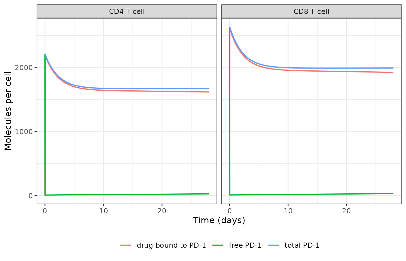
Replicates Figure S5 of Shchelokov 2023: dynamics of free, bound and total PD-1 on CD4 and CD8 T cells after a single 240 mg infusion.
Check 4: the four RO equations diverge in the published order
Figure 4 of the paper compares the four readouts for a single flat 240 mg infusion, the approved nivolumab dose. The Results state the ordering plainly: “reported occupancy level and its apparent maintenance depend on the strategy of RO assessment and increase in raw: equation 3 < equation 4 < equation 2 < equation 1”. Equations 1, 2 and 4 give near-complete and prolonged occupancy; Equation 3 alone produces the distinctive sharp peak followed by a slowly decaying plateau.
ro240 <- solve_typical(dose_mg = 240, wt = 80, tobs = seq(0, 672, by = 0.25))
#> ℹ parameter labels from comments will be replaced by 'label()'
#> Warning: No sigma parameters in the model
#> ℹ omega/sigma items treated as zero: 'etalvc', 'etalcl', 'etalvp', 'etakdeg', 'etabl_pd1_cd4', 'etabl_pd1_cd8', 'etaf_expression'

ro_long <- ro240 |>
  dplyr::select(time, ro1_cd8, ro2_cd8, ro3_cd8, ro4_cd8) |>
  tidyr::pivot_longer(-time, names_to = "eq", values_to = "ro") |>
  dplyr::mutate(eq = c(
    ro1_cd8 = "Eq 1: free, baseline",
    ro2_cd8 = "Eq 2: free, each time point",
    ro3_cd8 = "Eq 3: bound, baseline",
    ro4_cd8 = "Eq 4: bound, each time point"
  )[.data$eq])

ggplot(ro_long, aes(time / 24, ro, colour = eq)) +
  geom_line(linewidth = 0.7) +
  coord_cartesian(ylim = c(0, 105)) +
  labs(x = "Time (days)", y = "Receptor occupancy (%)", colour = NULL) +
  theme_bw() + theme(legend.position = "bottom")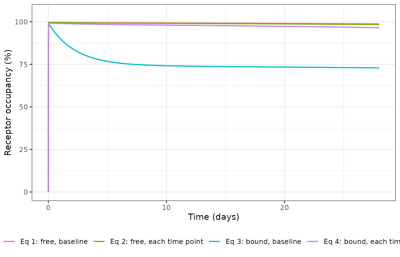
Replicates Figure 4 of Shchelokov 2023: PD-1 occupancy on CD8 T cells after a single 240 mg infusion, by RO assessment strategy.
ord <- ro240 |>
  dplyr::filter(.data$time >= 24) |>
  dplyr::summarise(
    dplyr::across(c(ro1_cd8, ro2_cd8, ro3_cd8, ro4_cd8), mean)
  )
knitr::kable(round(ord, 2), caption = "Mean occupancy over days 1-28 by equation.")| ro1_cd8 | ro2_cd8 | ro3_cd8 | ro4_cd8 |
|---|---|---|---|
| 99.19 | 98.94 | 74.96 | 97.72 |
# Typical-value solve, so the ordering is deterministic and can be asserted
# exactly rather than as a trend.
stopifnot(all(ro240$ro3_cd8[ro240$time >= 24] < ro240$ro4_cd8[ro240$time >= 24]))
stopifnot(all(ro240$ro4_cd8[ro240$time >= 24] < ro240$ro2_cd8[ro240$time >= 24]))
stopifnot(all(ro240$ro2_cd8[ro240$time >= 24] < ro240$ro1_cd8[ro240$time >= 24]))

# Equation 3 shows a sharp peak within the first day, then a lower plateau;
# equations 1, 2 and 4 stay near-complete throughout (Results, Figure 4).
peak3   <- max(ro240$ro3_cd8)
t_peak3 <- ro240$time[which.max(ro240$ro3_cd8)]
stopifnot(
  t_peak3 <= 24,
  peak3 - mean(ro240$ro3_cd8[ro240$time >= 168]) > 15,
  min(ro240$ro1_cd8[ro240$time >= 1]) > 90,
  min(ro240$ro2_cd8[ro240$time >= 1]) > 90,
  min(ro240$ro4_cd8[ro240$time >= 1]) > 90
)
Check 5: with no enhanced internalization the equations collapse in pairs
The paper’s closing simulation sets the internalization rate of bound
receptor equal to the degradation rate of free receptor – that is,
Expression = 1 – and reports that the baseline- and
time-point-normalized equations then agree within each assay format,
while a residual gap remains between the free and bound
formats. That gap is not an artifact: the bound strategy counts antibody
molecules, [mAb:R] + [R:mAb:R], whereas the total-receptor
denominator counts receptors, so a ternary complex contributes one to
the numerator and two to the denominator.
mod_noint <- rxode2::ini(rxode2::zeroRe(mod), f_expression = 1)
#> ℹ parameter labels from comments will be replaced by 'label()'
#> Warning: No sigma parameters in the model
#> ℹ change initial estimate of `f_expression` to `1`
ev_noint <- make_events(240, wt = 80, tobs = seq(0, 672, by = 1))
noint <- rxode2::rxSolve(mod_noint, ev_noint, returnType = "data.frame",
                         useLinCmt = FALSE)
#> ℹ omega/sigma items treated as zero: 'etalvc', 'etalcl', 'etalvp', 'etakdeg', 'etabl_pd1_cd4', 'etabl_pd1_cd8', 'etaf_expression'

cmp <- noint |>
  dplyr::filter(.data$time >= 1) |>
  dplyr::summarise(
    max_gap_eq1_eq2 = max(abs(.data$ro1_cd8 - .data$ro2_cd8)),
    max_gap_eq3_eq4 = max(abs(.data$ro3_cd8 - .data$ro4_cd8)),
    total_pd1_fold  = max(abs(.data$pd1_total_cd8 / p[["bl_pd1_cd8"]] - 1)),
    mean_free_eq1   = mean(.data$ro1_cd8),
    mean_bound_eq3  = mean(.data$ro3_cd8)
  )
knitr::kable(signif(cmp, 4),
caption = "Expression = 1: the paired equations collapse, the free/bound gap does not.")| max_gap_eq1_eq2 | max_gap_eq3_eq4 | total_pd1_fold | mean_free_eq1 | mean_bound_eq3 |
|---|---|---|---|---|
| 0 | 0 | 0 | 98.97 | 97.43 |
stopifnot(
  cmp$total_pd1_fold  < 1e-6, # no downmodulation, so total receptor is flat
  cmp$max_gap_eq1_eq2 < 1e-6, # Figure S6 A
  cmp$max_gap_eq3_eq4 < 1e-6, # Figure S6 B
  cmp$mean_free_eq1 > cmp$mean_bound_eq3 # Figure S6 C/D: the residual gap
)
Check 6: trough occupancy versus dose (Figure 2)
Figure 2 plots trough RO measured by Equation 3 at day 56 of Q2W dosing across 0.1 to 10 mg/kg, against the observed data of Topalian 2012. The Results describe the model curve as rising “from 60 to 70%”.
Body weights are sampled from the Bajaj 2017 demographics, truncated to that paper’s model-application range; Shchelokov 2023 does not state the virtual population’s weight distribution.
# set.seed() seeds R's RNG for the weight draw only. rxode2's own streams are
# partitioned per solver thread, so the simulated cohort differs between a
# 2-core CI runner and a 16-thread workstation. Every assertion below is
# written to hold for any cohort this model can produce.
set.seed(20230101)
n_arm <- 200L
wt <- pmin(pmax(rnorm(n_arm, mean = 79.1, sd = 19.3), 34.1), 168.2)

trough <- lapply(seq_along(doses_mgkg), function(k) {
  ev <- make_events(
    dose_mg = doses_mgkg[k] * wt, wt = wt, tobs = c(0, 1344),
    ii = 336, addl = 3L, id_offset = (k - 1L) * n_arm
  )
  rxode2::rxSolve(mod, ev, returnType = "data.frame", useLinCmt = FALSE) |>
    dplyr::filter(abs(.data$time - 1344) < 1e-6) |>
    dplyr::mutate(dose_mgkg = doses_mgkg[k])
}) |> dplyr::bind_rows()
#> ℹ parameter labels from comments will be replaced by 'label()'

trough_summary <- trough |>
  dplyr::group_by(dose_mgkg) |>
  dplyr::summarise(
    lo  = quantile(.data$ro3_cd8, 0.025),
    med = median(.data$ro3_cd8),
    hi  = quantile(.data$ro3_cd8, 0.975),
    .groups = "drop"
  )

# Read from Figure 2 of the paper (blue "Model" symbols, median with interval).
fig2 <- data.frame(
  dose_mgkg = doses_mgkg,
  paper_median = c(59, 67, 70, 72, 72),
  paper_lo = c(43, 47, 49, 49, 49),
  paper_hi = c(87, 99, 105, 106, 107)
)

ggplot(trough_summary, aes(factor(dose_mgkg), med)) +
  geom_pointrange(aes(ymin = lo, ymax = hi, colour = "This package"),
                  position = position_nudge(x = 0.11)) +
  geom_pointrange(
    data = fig2,
    aes(factor(dose_mgkg), paper_median, ymin = paper_lo, ymax = paper_hi,
        colour = "Shchelokov 2023 Fig. 2"),
    position = position_nudge(x = -0.11)
  ) +
  labs(x = "Dose (mg/kg Q2W)", y = "Trough occupancy at day 56, Eq. 3 (%)",
       colour = NULL) +
  theme_bw() + theme(legend.position = "bottom")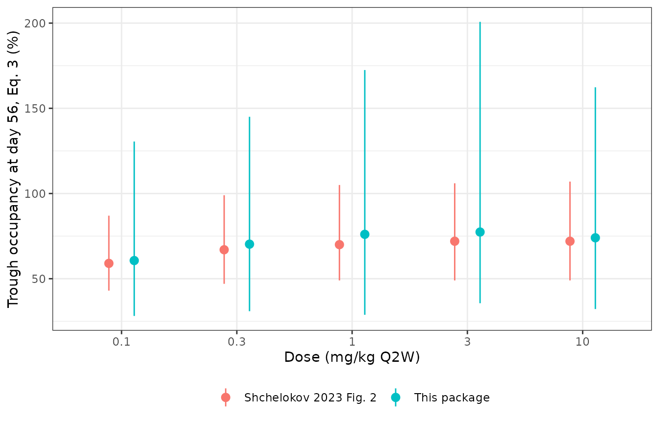
Replicates Figure 2 of Shchelokov 2023: trough PD-1 occupancy (Equation 3) at day 56 of Q2W dosing.
trough_summary |>
  dplyr::left_join(fig2, by = "dose_mgkg") |>
  dplyr::mutate(median_diff = .data$med - .data$paper_median) |>
  dplyr::select(dose_mgkg, med, paper_median, median_diff, lo, hi, paper_lo, paper_hi) |>
  dplyr::rename(
    "Dose (mg/kg)" = dose_mgkg, "Median, this package (%)" = med,
    "Median, Fig. 2 (%)" = paper_median, "Difference (pp)" = median_diff,
    "2.5th, this package" = lo, "97.5th, this package" = hi,
    "2.5th, Fig. 2" = paper_lo, "97.5th, Fig. 2" = paper_hi
  ) |>
knitr::kable(digits = 1, caption = "Trough RO (Eq. 3) at day 56 versus Figure 2.")| Dose (mg/kg) | Median, this package (%) | Median, Fig. 2 (%) | Difference (pp) | 2.5th, this package | 97.5th, this package | 2.5th, Fig. 2 | 97.5th, Fig. 2 |
|---|---|---|---|---|---|---|---|
| 0.1 | 60.7 | 59 | 1.7 | 28.1 | 130.5 | 43 | 87 |
| 0.3 | 70.3 | 67 | 3.3 | 30.9 | 145.0 | 47 | 99 |
| 1.0 | 76.0 | 70 | 6.0 | 28.8 | 172.5 | 49 | 105 |
| 3.0 | 77.4 | 72 | 5.4 | 35.6 | 200.7 | 49 | 106 |
| 10.0 | 74.0 | 72 | 2.0 | 32.2 | 162.3 | 49 | 107 |
md <- trough_summary$med
# Cohort-derived, so bounded on the centre only, with headroom. The paper's own
# claim is a rise "from 60 to 70%"; a mis-transcribed clearance, dose, receptor
# baseline or Expression value moves these medians by tens of points.
stopifnot(
  md[1] > 45, md[1] < 72,                       # 0.1 mg/kg, Fig. 2 reads ~59%
  md[length(md)] > 60, md[length(md)] < 85,     # 10 mg/kg, Fig. 2 reads ~72%
  md[length(md)] > md[1],                       # occupancy rises with dose
  median(abs(md - fig2$paper_median)) < 8
)
Check 7: single-dose profiles (Figures S2 and S3)
Figure S2 reports peak occupancy of 80-90% at the end of infusion with a sustained plateau near 70% after single doses of 0.3 to 10 mg/kg, and Figure S3 reports that occupancy persists with an apparent half-life of roughly 150 days after 10 mg/kg.
single <- lapply(c(0.3, 1, 3, 10), function(d) {
  solve_typical(dose_mg = d * 80, wt = 80,
                tobs = sort(unique(c(seq(0, 24, by = 0.25),
                                     seq(26, 24 * 300, by = 6))))) |>
    dplyr::mutate(dose_mgkg = d)
}) |> dplyr::bind_rows()
#> ℹ parameter labels from comments will be replaced by 'label()'
#> Warning: No sigma parameters in the model
#> ℹ omega/sigma items treated as zero: 'etalvc', 'etalcl', 'etalvp', 'etakdeg', 'etabl_pd1_cd4', 'etabl_pd1_cd8', 'etaf_expression'
#> ℹ parameter labels from comments will be replaced by 'label()'
#> Warning: No sigma parameters in the model
#> ℹ omega/sigma items treated as zero: 'etalvc', 'etalcl', 'etalvp', 'etakdeg', 'etabl_pd1_cd4', 'etabl_pd1_cd8', 'etaf_expression'
#> ℹ parameter labels from comments will be replaced by 'label()'
#> Warning: No sigma parameters in the model
#> ℹ omega/sigma items treated as zero: 'etalvc', 'etalcl', 'etalvp', 'etakdeg', 'etabl_pd1_cd4', 'etabl_pd1_cd8', 'etaf_expression'
#> ℹ parameter labels from comments will be replaced by 'label()'
#> Warning: No sigma parameters in the model
#> ℹ omega/sigma items treated as zero: 'etalvc', 'etalcl', 'etalvp', 'etakdeg', 'etabl_pd1_cd4', 'etabl_pd1_cd8', 'etaf_expression'

ggplot(single, aes(time / 24, ro3_cd8, colour = factor(dose_mgkg))) +
  geom_line(linewidth = 0.7) +
  coord_cartesian(xlim = c(0, 300), ylim = c(0, 105)) +
  labs(x = "Time (days)", y = "Occupancy, Eq. 3 (%)", colour = "Dose (mg/kg)") +
  theme_bw() + theme(legend.position = "bottom")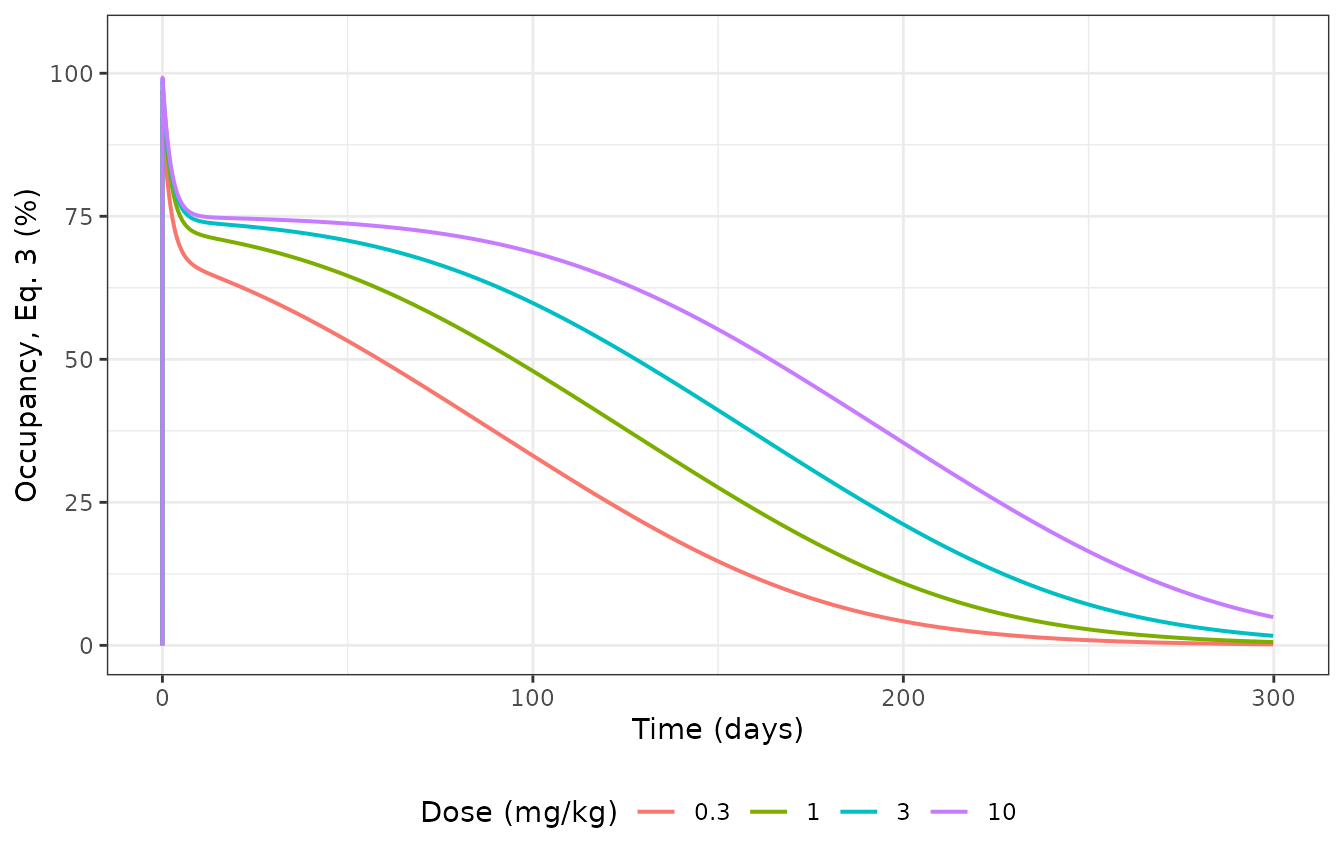
Replicates Figures S2 and S3 of Shchelokov 2023: Equation 3 occupancy on CD8 T cells after a single dose.
single_summary <- single |>
  dplyr::group_by(dose_mgkg) |>
  dplyr::summarise(
    peak = max(.data$ro3_cd8),
    t_peak_h = .data$time[which.max(.data$ro3_cd8)],
    plateau_d28 = .data$ro3_cd8[which.min(abs(.data$time - 672))],
    ro_d150 = .data$ro3_cd8[which.min(abs(.data$time - 24 * 150))],
    .groups = "drop"
  )
knitr::kable(single_summary, digits = 1,
caption = "Single-dose Equation 3 occupancy, typical value.")| dose_mgkg | peak | t_peak_h | plateau_d28 | ro_d150 |
|---|---|---|---|---|
| 0.3 | 92.2 | 1.5 | 60.6 | 14.7 |
| 1.0 | 96.9 | 1.2 | 69.1 | 27.6 |
| 3.0 | 98.6 | 1.2 | 72.9 | 41.1 |
| 10.0 | 99.2 | 1.0 | 74.5 | 55.2 |
# Typical-value solve. Peak is at the end of the 1 h infusion; the plateau
# approaches the 100 * Expression = 75.2% ceiling from Check 3 as dose rises.
stopifnot(
  all(single_summary$t_peak_h <= 2),
  all(single_summary$plateau_d28 > 55), all(single_summary$plateau_d28 < 76),
  # Figure S3: occupancy is still around half its peak at ~150 days.
  single_summary$ro_d150[single_summary$dose_mgkg == 10] > 40
)
Assumptions and deviations
-
ref_wt(80 kg) is not printed in the lead paper. Equation 5 normalizes body weight toBW_REFbut never gives its value. The entire PK block, including both body-weight exponents, is taken verbatim from Bajaj 2017, whose reference weight is 80 kg (Bajaj 2017 Table 1 footnote a);Vc = 3.63 LandCL = 9.4 mL/hare that paper’s typical values at 80 kg, so 80 kg is the only weight at which this model reproduces Table 1. Inherited from the upstream source, not from the lead paper. -
mw_mab(146 kDa) is not printed in the lead paper. The binding terms consume a nM antibody concentration while the PK module carries mass, so a molar mass is required to link them. The value is the calculated molecular mass in the OPDIVO US prescribing information (FDA 125554s112, 2022, Section 11), which is reference 12 of the lead paper. Not from the lead paper. -
The “Source” column of Table 1 is off by four for three
rows. Table 1 cites reference 23 for the PK block, 27 for
kdegand 28 forSAcell. Those superscripts are stale: the PK values match reference 27 (Bajaj 2017) exactly –Vc = 3.63 L,CL = 9.4 mL/h,Vp = 2.78 L,Q = 32.1 mL/h,Vc_BW = 0.597,CL_BW = 0.566and the variances 0.123 / 0.123 / 0.258 are Bajaj 2017’s Table 1 verbatim;kdeg = 0.01402 1/hisln(2)/49.4 h, the 49.5-hour PD-1 half-life of reference 31 (Lassman 2021); andSAcellis a cell surface area derived from spherical cell volume, reference 32 (Chapman 1981). All three shifts are +4, and every affected superscript is at least 19, so four references appear to have been inserted after the table was written. Rows citing references 14, 16 and 18 are consistent with the text and are unaffected. The Methods text, not the table’s superscripts, was used for provenance. -
Infusion duration. The paper says “zero-order IV
infusion” without a duration. The vignette uses 60 minutes, the duration
used in the trials the model is evaluated against (OPDIVO US prescribing
information, Section 14). The model itself takes the duration from the
event table’s
ratecolumn and makes no assumption. -
Which T-cell subset the published RO figures refer
to. Figures 2, 3 and 4 are labelled only “PD-1 occupancy”; only
Figure S5 separates CD4 from CD8. The model therefore emits all four RO
equations for both subsets (
ro1_cd4…ro4_cd8) and the vignette plots CD8. The two subsets differ only in baseline receptor count and their occupancy curves are nearly identical, so this choice does not affect any conclusion. -
The simulated 95% interval in Figure 2 is wider than the one
drawn in the paper. This is a real, reproducible disagreement
and it is not tuned away. Check 3 shows that the plateau of Equation 3
is exactly
100 * Expression, so the spread of trough RO is, to a very good approximation, the spread ofExpressionitself. Table 1 givesomega^2(Expression) = 0.218, which puts the 95% interval of a log-normal centred at 0.752 at roughly 30% to 188% – which is what this package simulates. Figure 2 draws an interval of about 49% to 107%, which corresponds instead toomega^2near 0.04 (equivalently, to reading 0.218 as a coefficient of variation rather than as a variance). The tabulated variance was preferred, because the same column’s PK entries (0.123, 0.123, 0.258) are unambiguously the variances of Bajaj 2017 and it would be inconsistent to read one column two ways. The medians, which are unaffected by this choice, reproduce Figure 2 closely. - Single-dose peak occupancy runs a little high. The Results describe Figure S2 as showing “a peak occupancy around 80-90% at the end of infusion”. The typical-value solve here peaks at 92% (0.3 mg/kg) to 99% (10 mg/kg), reported in the Check 7 table. The plateau, which is the quantity the paper actually argues from, matches: 61% to 75% against a stated “sustainable plateau occupancy of 70%”. The peak is the most transient point of the whole profile and the most sensitive to the infusion duration the paper does not state, and Figure S2 plots a cohort median rather than a typical-value solve, so the gap is not evidence of a transcription error. The Check 7 assertions therefore bound the plateau and the time-of-peak, not the peak height.
- Residual error. None is reported and none is encoded. The paper is a forward-simulation study; its intervals come from the inter-individual distributions alone.
-
No estimation. Every
ini()entry, including every variance, isfixed(), because Shchelokov 2023 fitted nothing – each value is carried from a cited source. Re-fitting this model to data would require unfixing the parameters of interest first. -
Not carried from Bajaj 2017. Shchelokov 2023 keeps
only Bajaj’s baseline clearance and body-weight covariate. Bajaj’s
time-varying (sigmoid
Emax) clearance, its eGFR, sex, ECOG and race effects, and its CL:Vc covariance are all absent from Table 1 and are therefore absent here. The full popPK model is packaged separately asBajaj_2017_nivolumab.