Omalizumab (Hayashi 2007) • nlmixr2lib

library(nlmixr2lib)
library(rxode2)
#> rxode2 5.1.2 using 2 threads (see ?getRxThreads)
#>   no cache: create with `rxCreateCache()`
library(dplyr)
#> 
#> Attaching package: 'dplyr'
#> The following objects are masked from 'package:stats':
#> 
#>     filter, lag
#> The following objects are masked from 'package:base':
#> 
#>     intersect, setdiff, setequal, union
library(tidyr)
library(ggplot2)
library(PKNCA)
#> 
#> Attaching package: 'PKNCA'
#> The following object is masked from 'package:stats':
#> 
#>     filter

Omalizumab–IgE binding population PK/PD model

Omalizumab is a humanized anti-IgE IgG1 monoclonal antibody used in moderate-to-severe atopic asthma. It interrupts the allergic cascade by binding free serum IgE, lowering its concentration, and downmodulating FcεRI on basophils and mast cells. Hayashi et al. (2007) developed a mechanism-based population PK/PD model in 202 Japanese subjects (single- and multiple-dose studies 1101 and 1305) that describes three serum entities — free omalizumab, free IgE, and the omalizumab–IgE complex — each with their own clearance and volume of distribution, coupled by an instantaneous-equilibrium binding step (law of mass action) with a concentration-dependent dissociation constant. Body weight modifies omalizumab CL and Vd; baseline IgE modifies IgE CL and IgE production rate. The model was externally validated against 531 White patients (studies 007/008/009).

Citation: Hayashi N, Tsukamoto Y, Sallas WM, Lowe PJ. A mechanism-based binding model for the population pharmacokinetics and pharmacodynamics of omalizumab. Br J Clin Pharmacol. 2007;63(5):548-561. doi:10.1111/j.1365-2125.2006.02803.x (PMID 17096680).
Article: https://doi.org/10.1111/j.1365-2125.2006.02803.x
PMID: 17096680

Population

The model-building dataset comprises 202 Japanese subjects from two clinical studies (Hayashi 2007 Table 1):

Study	Indication	n (used)	Design	Body weight (kg)	Baseline IgE (ng/mL)
1101	Healthy atopic volunteers	48	Single SC dose 75–375 mg	62.5 ± 6.4 (51–79)	811 ± 473 (204–2143)
1305	Seasonal allergic rhinitis (Japan)	154	Multiple SC dosing per the body-weight × IgE table (Table 2)	60.5 ± 10.2 (42–101)	373 ± 317 (53–1316)

A total of 3192 observation records (1037 omalizumab, 1191 total IgE, 964 free IgE) were included; 275 free-IgE values above the 150 ng/mL upper limit of quantification were excluded. The same metadata is available programmatically through readModelDb("Hayashi_2007_omalizumab")$population.

Source trace

Per-parameter origin is recorded as in-file comments next to each ini() entry in inst/modeldb/specificDrugs/Hayashi_2007_omalizumab.R. The table collects them for review.

Equation / parameter	Value (paper)	Value (file)	Source
`lka` (SC absorption rate)	0.0200 1/h	log(0.0200·24) 1/d	Table 3
`lcl` (apparent CL of free omalizumab at 61.1 kg)	7.32 mL/h	log(0.00732·24) L/d	Table 3
`ldcl_complex` (apparent excess CL of complex)	5.86 mL/h	log(0.00586·24) L/d	Table 3
`lcl_ige` (apparent CL of free IgE at 482.4 ng/mL)	71.0 mL/h	log(0.071·24) L/d	Table 3
`lvc` (apparent V of omalizumab and IgE at 61.1 kg)	5900 mL	log(5.9) L	Table 3 (V_E/f = V_X/f, footnote ‡)
`lvc_complex` (apparent V of complex)	3630 mL	log(3.63) L	Table 3
`lp_ige` (apparent IgE production rate at 482.4 ng/mL)	30.3 µg/h (= 0.1595 nmol/h)	log(0.1595·24) nmol/d	Table 3, footnote †
`lkd0` (Kd at X_TX = X_TE)	1.07 nM	log(1.07) nM	Table 3
`e_wt_cl` (BW exponent on CL_X)	0.911	0.911	Table 3
`e_wt_vc` (BW exponent on V_X)	0.658	0.658	Table 3
`e_ige_cl_ige` (IgE0 exponent on CL_E)	−0.281	−0.281	Table 3
`e_ige_p_ige` (IgE0 exponent on P_E)	0.657	0.657	Table 3
`alpha` (concentration dependence on Kd)	0.157	0.157	Table 3
`etalka`	CV 39.9%	ω² = 0.14773	Table 3
`etalcl`	CV 20.3%	ω² = 0.04042	Table 3
`etaldcl_complex`	CV 34.9%	ω² = 0.11488	Table 3
`etalvc` (shared by V_X and V_E)	CV 13.0%	ω² = 0.01679	Table 3
`etalvc_complex`	CV 25.0%	ω² = 0.06062	Table 3
`etalcl_ige + etalp_ige` (block; r = 0.968)	CV 25.3% / 23.1%	ω² = 0.06205, cov 0.05496, ω² = 0.05197	Table 3
`propSd` / `propSd_totalIgE` / `propSd_freeIgE` (Y = F·exp(ε))	σ ≈ 16.7% / 21.1% / 21.8%	0.167 / 0.211 / 0.218	Table 3
Eq. dX_SC/dt = −ka·X_SC + f·D·δ(t−tD)	n/a	n/a	Methods, page 552
Eq. dX_TX/dt = ka·X_SC − CL_X·C_fX − CL_C·C_C	n/a	n/a	Methods, page 552
Eq. dX_TE/dt = P_E − CL_E·C_fE − CL_C·C_C	n/a	n/a	Methods, page 552
Quadratic X_C = ½{S − √(S² − 4·X_TX·X_TE)}, S = X_TX + X_TE + Kd·V_X·V_E/V_C	n/a	n/a	Methods, page 552
Concentration-dependent Kd = Kd0·(X_TX/X_TE)^α	n/a	n/a	“The dissociation constant”, page 552
Power covariates: CL_X, V_X on (WT/61.1); CL_E, P_E on (IgE0/482.4)	n/a	n/a	Page 555 equations
MW(omalizumab) = 150 kDa; MW(IgE) = 190 kDa	150 / 190 kDa	150 / 190 kDa	Methods, page 552
Subcutaneous bioavailability used to translate apparent values to absolute	f = 0.62 (ref [28])	not encoded; CL/f and V/f in `ini()`	Discussion, page 559

Virtual cohort

Original observed data are not publicly available. The cohort below reproduces the four single-dose groups of study 1101 (75, 150, 300, and 375 mg SC) — the only design with a dense sampling schedule (Hayashi 2007 Methods, page 549). Body weight and baseline IgE are sampled from the study-1101 distribution (mean 62.5 kg ± 6.4 kg; mean 811 ng/mL ± 473 ng/mL, log-normal).

set.seed(20070501L) # paper publication month YYYYMM01

study_1101_doses <- c(75, 150, 300, 375)
n_per_dose       <- 12L

make_cohort <- function(n, dose_mg, id_offset = 0L) {
  data.frame(
    id    = id_offset + seq_len(n),
    dose  = dose_mg,
    WT    = pmax(45, pmin(80, rnorm(n, mean = 62.5, sd = 6.4))),
    IGE   = pmax(200, pmin(2200,
              exp(rnorm(n, mean = log(811) - 0.5 * log(1 + (473 / 811)^2),
                          sd = sqrt(log(1 + (473 / 811)^2))))))
  )
}

cohorts <- bind_rows(lapply(seq_along(study_1101_doses), function(i) {
  make_cohort(n_per_dose, study_1101_doses[i],
              id_offset = (i - 1L) * n_per_dose)
}))

obs_times <- c(0, 0.5, 1, 2, 4, 7, 10, 14, 28, 42, 56, 70, 84) # days, study 1101 schedule

events <- cohorts |>
  rowwise() |>
  do({
    row <- .
    et_obj <- rxode2::et(time = 0, amt = row$dose, cmt = "depot") |>
      rxode2::et(obs_times, cmt = "Cc")
    et_obj$id    <- row$id
    et_obj$WT    <- row$WT
    et_obj$IGE   <- row$IGE
    et_obj$dose  <- row$dose
    et_obj
  }) |>
  ungroup() |>
  as.data.frame()

stopifnot(!anyDuplicated(unique(events[, c("id", "time", "evid")])))

Simulation

mod <- readModelDb("Hayashi_2007_omalizumab")
sim <- rxode2::rxSolve(mod, events = events,
                       keep = c("dose", "WT", "IGE"),
                       returnType = "data.frame", addDosing = FALSE)
#> ℹ parameter labels from comments will be replaced by 'label()'
sim$dose_label <- factor(paste0(sim$dose, " mg"),
                         levels = paste0(study_1101_doses, " mg"))

Replicate published Figure 3 — single-dose profiles by dose level

Hayashi 2007 Figure 3 shows individual observed serum concentrations of omalizumab, total IgE, and free IgE in study 1101 over 84 days, with 80% prediction intervals. We reproduce the cohort means with 80% prediction intervals from the simulated population.

sim |>
  group_by(time, dose_label) |>
  summarise(
    Q10 = quantile(Cc, 0.10, na.rm = TRUE),
    Q50 = quantile(Cc, 0.50, na.rm = TRUE),
    Q90 = quantile(Cc, 0.90, na.rm = TRUE),
    .groups = "drop"
  ) |>
  ggplot(aes(time, Q50)) +
  geom_ribbon(aes(ymin = Q10, ymax = Q90), alpha = 0.25) +
  geom_line() +
  facet_wrap(~ dose_label, scales = "free_y") +
  labs(x = "Time (days)", y = "Total omalizumab (µg/mL)",
       title = "Hayashi 2007 Figure 3, omalizumab panel",
       caption = "Lines: median; ribbon: 10th–90th percentile from 12 simulated subjects per dose.")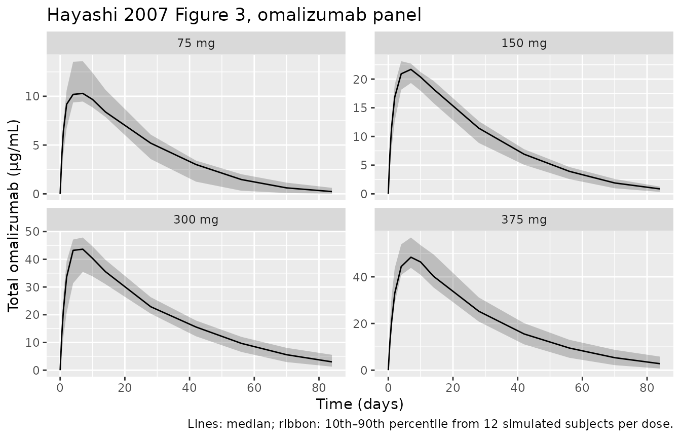

Replicates Figure 3 of Hayashi 2007 (top row, omalizumab vs time by single-dose group, study 1101).

sim |>
  group_by(time, dose_label) |>
  summarise(
    Q10 = quantile(freeIgE, 0.10, na.rm = TRUE),
    Q50 = quantile(freeIgE, 0.50, na.rm = TRUE),
    Q90 = quantile(freeIgE, 0.90, na.rm = TRUE),
    .groups = "drop"
  ) |>
  ggplot(aes(time, Q50)) +
  geom_ribbon(aes(ymin = Q10, ymax = Q90), alpha = 0.25) +
  geom_line() +
  facet_wrap(~ dose_label) +
  scale_y_log10() +
  geom_hline(yintercept = 12, lty = 2, colour = "grey40") +
  geom_hline(yintercept = 21, lty = 2, colour = "grey40") +
  labs(x = "Time (days)", y = "Free IgE (ng/mL, log scale)",
       title = "Hayashi 2007 Figure 3, free-IgE panel",
       caption = "Dashed grey lines indicate the 12–21 ng/mL clinical-efficacy band cited in Hayashi 2007.")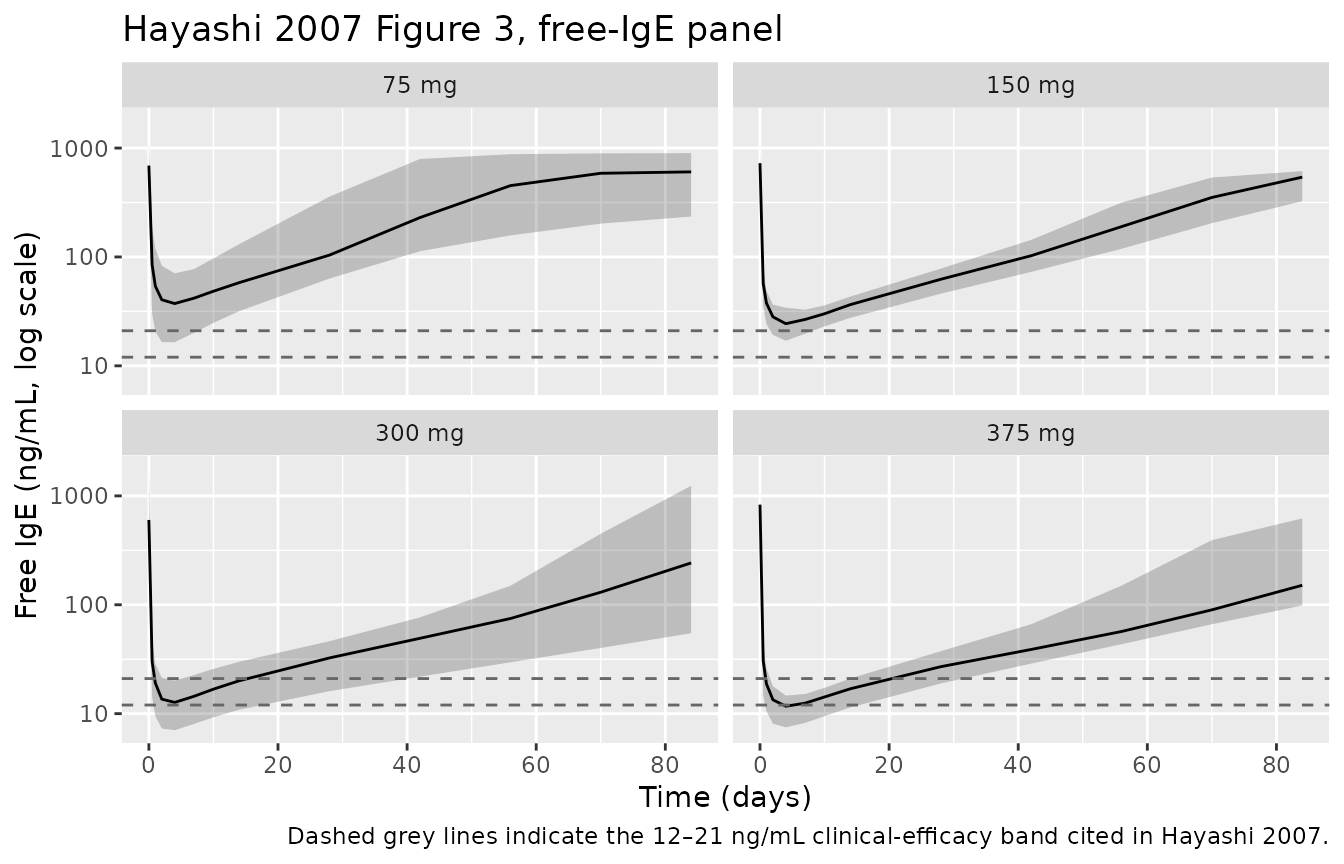

Replicates Figure 3 of Hayashi 2007 (free IgE vs time by single-dose group, study 1101).

sim |>
  group_by(time, dose_label) |>
  summarise(
    Q10 = quantile(totalIgE, 0.10, na.rm = TRUE),
    Q50 = quantile(totalIgE, 0.50, na.rm = TRUE),
    Q90 = quantile(totalIgE, 0.90, na.rm = TRUE),
    .groups = "drop"
  ) |>
  ggplot(aes(time, Q50)) +
  geom_ribbon(aes(ymin = Q10, ymax = Q90), alpha = 0.25) +
  geom_line() +
  facet_wrap(~ dose_label) +
  labs(x = "Time (days)", y = "Total IgE (ng/mL)",
       title = "Hayashi 2007 Figure 3, total-IgE panel")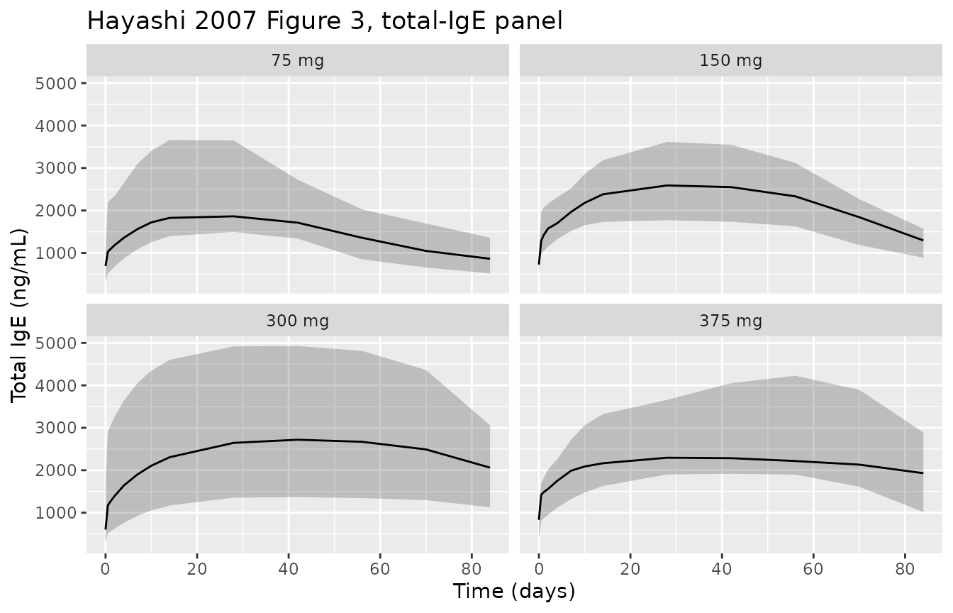

Replicates Figure 3 of Hayashi 2007 (total IgE vs time by single-dose group, study 1101).

PKNCA validation — omalizumab

PKNCA computes Cmax, Tmax, AUC(0,∞), and terminal half-life on the simulated total-omalizumab profile. Hayashi 2007 reports a noncompartmental terminal half-life of 18.2 days for total omalizumab in study 1101 (Discussion, page 558) and a model-derived half-life of 23 days for free omalizumab. The compartmental Cc output is total omalizumab (free + complex), so the NCA t½ is expected to land between those two values.

sim_nca <- sim |>
  filter(!is.na(Cc)) |>
  select(id, time, Cc, dose_label)

dose_df <- events |>
  filter(evid == 1) |>
  mutate(dose_label = factor(paste0(amt, " mg"),
                             levels = paste0(study_1101_doses, " mg"))) |>
  select(id, time, amt, dose_label)

conc_obj <- PKNCA::PKNCAconc(sim_nca, Cc ~ time | dose_label + id)
dose_obj <- PKNCA::PKNCAdose(dose_df, amt ~ time | dose_label + id)

intervals <- data.frame(
  start      = 0,
  end        = Inf,
  cmax       = TRUE,
  tmax       = TRUE,
  aucinf.obs = TRUE,
  half.life  = TRUE
)

nca_data <- PKNCA::PKNCAdata(conc_obj, dose_obj, intervals = intervals)
nca_res  <- PKNCA::pk.nca(nca_data)
nca_summary <- summary(nca_res)
knitr::kable(nca_summary, caption = "Simulated NCA parameters by single-dose group (study 1101).")

Simulated NCA parameters by single-dose group (study 1101).
end	dose_label	N	cmax	tmax	half.life	aucinf.obs
Inf	75 mg	12	10.7 [13.0]	7.00 [4.00, 10.0]	11.8 [5.12]	332 [25.1]
Inf	150 mg	12	20.8 [16.1]	7.00 [4.00, 10.0]	14.8 [5.58]	745 [18.4]
Inf	300 mg	12	44.6 [14.0]	7.00 [4.00, 7.00]	17.9 [4.42]	1650 [13.8]
Inf	375 mg	12	49.9 [14.4]	7.00 [4.00, 10.0]	18.1 [4.87]	1810 [22.4]

Comparison against published values

Hayashi 2007 reports only a single global noncompartmental t½ for total omalizumab in study 1101 (18.2 days; Discussion, page 558) and the model-derived half-lives of free omalizumab (23 days) and IgE (2.4 days). The simulated terminal t½ for total omalizumab in the typical patient should sit between the two model-derived bounds (23 days for free omalizumab; faster for the complex due to ΔCL_C = 5.86 mL/h on top of CL_X = 7.32 mL/h). No per-dose NCA table is published, so a fully quantitative side-by-side comparison is not possible.

Mechanism check — typical-value pre-treatment steady state

Without drug, X_TE evolves under dX_TE/dt = P_E − CL_E·C_fE. The model’s typical-value pre-treatment steady-state free-IgE concentration is (P_E / CL_E) · MW_IgE = 426.8 ng/mL. The covariate reference value is 482.4 ng/mL — a small (~12%) intentional offset because P_E and CL_E are independently estimated and not constrained to reproduce IgE0 at steady state. With the model’s initial condition X_TE(0) = (IGE / MW_IgE)·V_E, free IgE starts at the observed baseline and drifts toward the model SS over the first few days when there is no drug; once dosing begins the binding kinetics dominate this small drift.

mod_typ <- rxode2::zeroRe(mod)
#> ℹ parameter labels from comments will be replaced by 'label()'
ev_nodose <- rxode2::et(seq(0, 30, by = 1), cmt = "Cc")
sim_nodose <- rxode2::rxSolve(mod_typ, events = ev_nodose,
                              params = c(WT = 61.1, IGE = 482.4),
                              returnType = "data.frame", addDosing = FALSE)
#> ℹ omega/sigma items treated as zero: 'etalka', 'etalcl', 'etaldcl_complex', 'etalvc', 'etalvc_complex', 'etalcl_ige', 'etalp_ige'
ggplot(sim_nodose, aes(time, freeIgE)) +
  geom_line() +
  geom_hline(yintercept = 482.4, lty = 2, colour = "grey40") +
  geom_hline(yintercept = (0.1595 / 0.071) * 190, lty = 3, colour = "grey40") +
  labs(x = "Time (days, no drug)", y = "Free IgE (ng/mL)",
       title = "Pre-treatment steady-state drift toward the model SS",
       caption = "Dashed: observed IgE0 = 482.4 ng/mL (initial). Dotted: model SS = P_E/CL_E·MW_IgE ≈ 426.8 ng/mL.")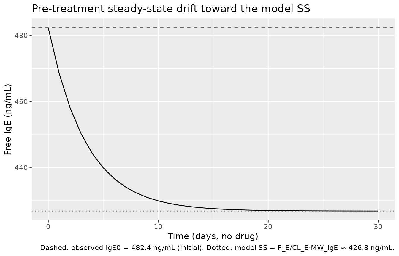

Assumptions and deviations

Bioavailability not encoded explicitly. The paper reports apparent parameters (CL_X/f, V_X/f, etc.) and notes f = 0.62 from a separate source (Discussion, page 559). The model file uses the apparent values directly with no f scaling on the dose, which faithfully reproduces the predicted measured concentrations in the original NONMEM fit. Absolute clearances and volumes can be recovered by multiplying the apparent values by 0.62.
Time unit conversion h → d. The paper reports CL and ka in 1/h, consistent with NONMEM convention. The model file converts to 1/day by multiplying each rate by 24, with the conversion shown in the ini() source-trace comment for every rate parameter. Half-lives derived from the converted values match the paper (23 days for free omalizumab, 2.4 days for IgE).
Residual error written as proportional rather than exact log-normal. Hayashi 2007 uses Y = F · exp(ε); for σ in the 0.17–0.22 range encountered here, Y ≈ F·(1 + ε), so a proportional error model with propSd = σ is faithful to within third-order ε terms. nlmixr2’s prop() keyword maps to this approximation; the alternative lnorm() parameterization could be used in future revisions.
V_E/f shared with V_X/f. Footnote ‡ of Table 3 states V_E/f was fixed equal to V_X/f because separate estimation did not converge. The model file enforces this by setting v_ige <- vc (same individual parameter, including the same etalvc IIV).
Concentration-dependent Kd at t = 0. With central (paper X_TX) = 0 at t = 0, Kd = Kd0·(0/total_target)^α = 0 for α > 0, S = total_target, and the negative root yields X_C = 0. This matches the physical expectation (no drug, no complex). After dosing begins central becomes strictly positive and the expression evaluates without numerical issues.
Compartment names. The paper’s X_TX (total omalizumab amount in serum, free + complex) maps to the canonical central compartment; X_TE (total IgE amount, free + complex) maps to total_target. This follows the canonical TMDD compartment names registered in references/naming-conventions.md for QSS-style total-amount parameterizations (Gibiansky 2008). The complex species is algebraically derived from the equilibrium relation rather than carried as a separate ODE state.
External validation cohort not modelled. The paper validates predictions against 531 White patients in studies 007/008/009 using the model fit to Japanese subjects only. The packaged model contains the Japanese-fit parameters; it does not encode separate White-cohort estimates because none were estimated by the authors.
Race recorded as Asian = 100%. Hayashi 2007 Table 1 enumerates 202 Japanese subjects in studies 1101 and 1305 with no other race groups in the model-building cohort; the population metadata records the cohort as 100% Asian (Japanese) accordingly.
Initial total_target uses observed IGE0, not the model SS. As described in the Mechanism-check section, initialising at IGE causes a small pre-treatment drift before binding dominates. Users wanting a steady-state initialisation can override inits = c(total_target = p_ige / cl_ige * v_ige) after computing p_ige, cl_ige, and v_ige for the cohort of interest.

Reproducibility

sessionInfo()
#> R version 4.6.0 (2026-04-24)
#> Platform: x86_64-pc-linux-gnu
#> Running under: Ubuntu 24.04.4 LTS
#> 
#> Matrix products: default
#> BLAS:   /usr/lib/x86_64-linux-gnu/openblas-pthread/libblas.so.3 
#> LAPACK: /usr/lib/x86_64-linux-gnu/openblas-pthread/libopenblasp-r0.3.26.so;  LAPACK version 3.12.0
#> 
#> locale:
#>  [1] LC_CTYPE=C.UTF-8       LC_NUMERIC=C           LC_TIME=C.UTF-8       
#>  [4] LC_COLLATE=C.UTF-8     LC_MONETARY=C.UTF-8    LC_MESSAGES=C.UTF-8   
#>  [7] LC_PAPER=C.UTF-8       LC_NAME=C              LC_ADDRESS=C          
#> [10] LC_TELEPHONE=C         LC_MEASUREMENT=C.UTF-8 LC_IDENTIFICATION=C   
#> 
#> time zone: UTC
#> tzcode source: system (glibc)
#> 
#> attached base packages:
#> [1] stats     graphics  grDevices utils     datasets  methods   base     
#> 
#> other attached packages:
#> [1] PKNCA_0.12.1          ggplot2_4.0.3         tidyr_1.3.2          
#> [4] dplyr_1.2.1           rxode2_5.1.2          nlmixr2lib_0.3.2.9000
#> 
#> loaded via a namespace (and not attached):
#>  [1] gtable_0.3.6          xfun_0.58             bslib_0.11.0         
#>  [4] lattice_0.22-9        vctrs_0.7.3           tools_4.6.0          
#>  [7] generics_0.1.4        parallel_4.6.0        tibble_3.3.1         
#> [10] symengine_0.2.11      pkgconfig_2.0.3       data.table_1.18.4    
#> [13] checkmate_2.3.4       RColorBrewer_1.1-3    S7_0.2.2             
#> [16] desc_1.4.3            RcppParallel_5.1.11-2 lifecycle_1.0.5      
#> [19] compiler_4.6.0        farver_2.1.2          textshaping_1.0.5    
#> [22] fontawesome_0.5.3     htmltools_0.5.9       sys_3.4.3            
#> [25] sass_0.4.10           yaml_2.3.12           crayon_1.5.3         
#> [28] pillar_1.11.1         pkgdown_2.2.0         jquerylib_0.1.4      
#> [31] whisker_0.4.1         openssl_2.4.1         cachem_1.1.0         
#> [34] nlme_3.1-169          qs2_0.2.2             tidyselect_1.2.1     
#> [37] digest_0.6.39         lotri_1.0.4           purrr_1.2.2          
#> [40] labeling_0.4.3        rxode2ll_2.0.14       fastmap_1.2.0        
#> [43] grid_4.6.0            cli_3.6.6             dparser_1.3.1-13     
#> [46] magrittr_2.0.5        withr_3.0.2           scales_1.4.0         
#> [49] backports_1.5.1       rmarkdown_2.31        otel_0.2.0           
#> [52] askpass_1.2.1         ragg_1.5.2            stringfish_0.19.0    
#> [55] memoise_2.0.1         evaluate_1.0.5        knitr_1.51           
#> [58] rex_1.2.2             PreciseSums_0.7       rlang_1.2.0          
#> [61] downlit_0.4.5         Rcpp_1.1.1-1.1        glue_1.8.1           
#> [64] xml2_1.5.2            jsonlite_2.0.0        R6_2.6.1             
#> [67] systemfonts_1.3.2     fs_2.1.0