Tafenoquine (Edstein 2001)
Source:vignettes/articles/Edstein_2001_tafenoquine.Rmd
Edstein_2001_tafenoquine.RmdModel and source
- Citation: Edstein MD, Kocisko DA, Brewer TG, Walsh DS, Eamsila C, Charles BG (2001). Population pharmacokinetics of the new antimalarial agent tafenoquine in Thai soldiers. British Journal of Clinical Pharmacology 52(6):663-670. doi:10.1046/j.0306-5251.2001.01482.x.
- Article: https://doi.org/10.1046/j.0306-5251.2001.01482.x
The package model can be loaded with:
mod_fn <- readModelDb("Edstein_2001_tafenoquine")
mod    <- rxode2::rxode2(mod_fn())
Population
Edstein 2001 fitted a one-compartment oral PK model to plasma tafenoquine concentrations from 135 male Thai soldiers (mean age 28.9 years, range 21-46; mean weight 60.3 kg, range 45-90) deployed on security operations along the Thai-Cambodian border (Edstein 2001 Table 1). All subjects were G6PD-normal and were pre-treated with artesunate (300 mg day 1, 120 mg days 2-3) plus 200 mg daily doxycycline for 7 days to clear any pre-existing parasitaemia. Two prophylactic regimens were studied:
- Monthly cohort (n = 104). A 400 mg loading dose of tafenoquine base daily for 3 days followed by 400 mg monthly for 5 consecutive months.
- Weekly cohort (n = 31). Subjects originally in the placebo arm who contracted malaria during the trial were re-treated with the same artesunate + doxycycline regime and then maintained on a 400 mg loading dose daily for 3 days followed by 400 mg weekly.
Doses were taken with food (cake and biscuits) and 80-100 mL water. Plasma tafenoquine was assayed by reversed-phase HPLC with fluorescence detection (LLOQ 10 ng/mL; interday / intraday CV <= 8.4 %, mean recovery 81 %). The population metadata recorded in the model file mirrors Table 1 of the source:
Source trace
The per-parameter origin is recorded next to each ini()
entry in
inst/modeldb/specificDrugs/Edstein_2001_tafenoquine.R. The
table below collects them in one place.
| Equation / parameter | Value | Source location |
|---|---|---|
lka (Ka) |
0.694 / h | Edstein 2001 Table 3 (theta_3) |
lcl (CL/F) |
3.20 L/h | Edstein 2001 Table 3 (theta_1) |
lvc (V/F) |
1820 L | Edstein 2001 Table 3 (theta_2) |
etalcl variance (CL/F) |
0.06204 (25.3 % CV) | Edstein 2001 Table 3 (omega_CL/F); omega^2 = log(0.253^2 + 1) |
etalvc variance (V/F) |
0.02167 (14.8 % CV) | Edstein 2001 Table 3 (omega_V/F); omega^2 = log(0.148^2 + 1) |
etalka variance (Ka) |
0.31791 (61.2 % CV) | Edstein 2001 Table 3 (omega_Ka); omega^2 = log(0.612^2 + 1) |
cov(etalcl, etalvc) |
0.0265 (rho ~ 0.71-0.72) | Edstein 2001 Table 3 (cov V/F, CL/F) via $OMEGA BLOCK(2); paper Results report rho = 0.71 |
propSd (residual) |
0.179 (17.9 % CV) | Edstein 2001 Table 3 (sigma) – exponential error model per Methods |
d/dt(depot), d/dt(central)
|
n/a | Methods ‘Population modelling’: one-compartment with first-order absorption and elimination |
| Concentration scaling x1000 | n/a | Dimensional analysis: dose in mg / V in L = mg/L = 1000 ng/mL (paper reports concentrations in ng/mL) |
| Excluded – WT, AGE on V/F; MAL on CL/F | n/a | Edstein 2001 Table 2 covariate model-development summary; Results adopt model no. 1 (no covariates) |
Virtual cohort
The original observed data are not publicly available. The figures below use virtual cohorts whose dose schedules match the published regimens. Because the final model has no covariates, the only per-subject variability comes from the random effects on CL/F, V/F, and Ka; the cohorts therefore share a single typical subject and differ only in dose schedule.
set.seed(20240101)

# Helper: dose schedule for a single subject. Returns a long-format event
# table covering dosing rows (evid = 1) and observation rows (evid = 0).
make_cohort <- function(n, dose_times_h, sample_times_h, treatment,
                        id_offset = 0L, amt_mg = 400) {
  dose_rows <- tidyr::expand_grid(
    id   = id_offset + seq_len(n),
    time = dose_times_h
  ) |>
    dplyr::mutate(
      amt  = amt_mg,
      evid = 1,
      cmt  = "depot"
    )
  obs_rows <- tidyr::expand_grid(
    id   = id_offset + seq_len(n),
    time = sample_times_h
  ) |>
    dplyr::mutate(
      amt  = 0,
      evid = 0,
      cmt  = "central"
    )
  dplyr::bind_rows(dose_rows, obs_rows) |>
    dplyr::arrange(id, time, dplyr::desc(evid)) |>
    dplyr::mutate(treatment = treatment)
}

# Monthly cohort: 400 mg daily x 3, then 400 mg every 28 days for 5 months
# (8 total doses). Follow-up through 1 month past the last dose per the
# study's '6 months chemosuppression + 1 month follow-up' window.
dose_times_monthly <- c(0, 24, 48,
                        c(28, 56, 84, 112, 140) * 24)
end_monthly <- max(dose_times_monthly) + 28 * 24  # 7 days short of full month
sample_times_monthly <- sort(unique(c(
  seq(0, 72, by = 1),                       # dense over loading period
  seq(72, end_monthly, by = 24)             # daily after loading
)))

# Weekly cohort: 400 mg daily x 3, then 400 mg every 7 days for 24 weeks.
dose_times_weekly <- c(0, 24, 48,
                       72 + seq(0, 24 * 7 - 1) * 24 * 7)
end_weekly <- max(dose_times_weekly) + 24 * 28
sample_times_weekly <- sort(unique(c(
  seq(0, 72, by = 1),                       # dense over loading period
  seq(72, end_weekly, by = 24)              # daily after loading
)))

events <- dplyr::bind_rows(
  make_cohort(50, dose_times_monthly, sample_times_monthly, "Monthly",
              id_offset =   0L),
  make_cohort(50, dose_times_weekly,  sample_times_weekly,  "Weekly",
              id_offset = 100L)
)

stopifnot(!anyDuplicated(unique(events[, c("id", "time", "evid")])))
Simulation
sim <- rxode2::rxSolve(mod, events = events, keep = c("treatment")) |>
  as.data.frame() |>
  dplyr::filter(!is.na(Cc))
For deterministic replication (typical-value profiles without between-subject variability), zero out the random effects:
Replicate published figures
# Replicates Figure 2a of Edstein 2001: individual plasma tafenoquine
# concentration vs time for monthly dosing.
sim |>
  dplyr::filter(treatment == "Monthly") |>
  dplyr::mutate(time_days = time / 24) |>
  ggplot(aes(time_days, Cc, group = id)) +
  geom_line(alpha = 0.25) +
  scale_y_log10() +
  labs(x = "Time (days)", y = "Plasma tafenoquine (ng/mL)",
       title = "Figure 2a -- Monthly prophylaxis (virtual cohort, n = 50)",
       caption = "Replicates Figure 2a of Edstein 2001 (individual profiles, monthly cohort).")
#> Warning in scale_y_log10(): log-10 transformation introduced infinite values.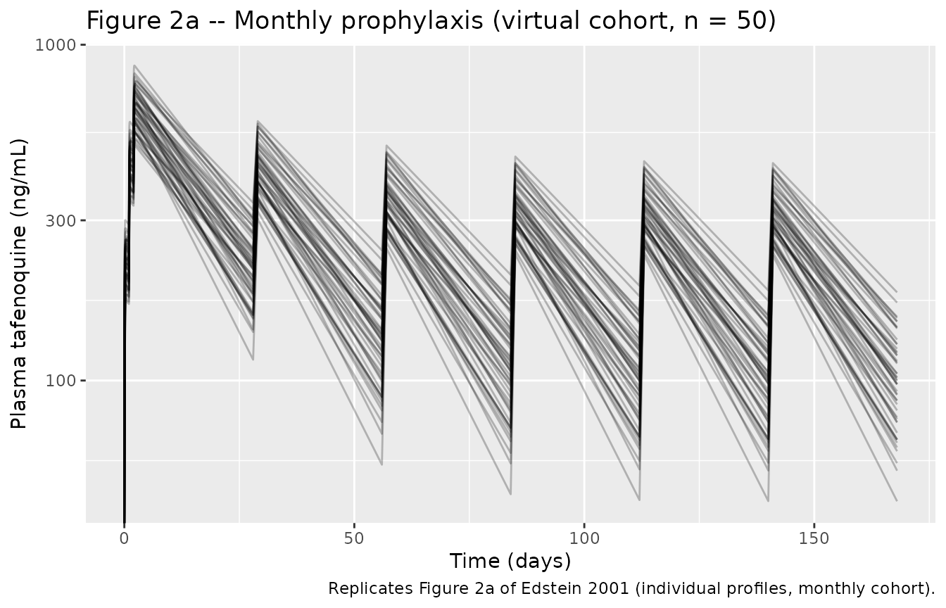
# Replicates Figure 2b of Edstein 2001: individual plasma tafenoquine
# concentration vs time for weekly dosing.
sim |>
  dplyr::filter(treatment == "Weekly") |>
  dplyr::mutate(time_days = time / 24) |>
  ggplot(aes(time_days, Cc, group = id)) +
  geom_line(alpha = 0.25) +
  scale_y_log10() +
  labs(x = "Time (days)", y = "Plasma tafenoquine (ng/mL)",
       title = "Figure 2b -- Weekly prophylaxis (virtual cohort, n = 50)",
       caption = "Replicates Figure 2b of Edstein 2001 (individual profiles, weekly cohort).")
#> Warning in scale_y_log10(): log-10 transformation introduced infinite values.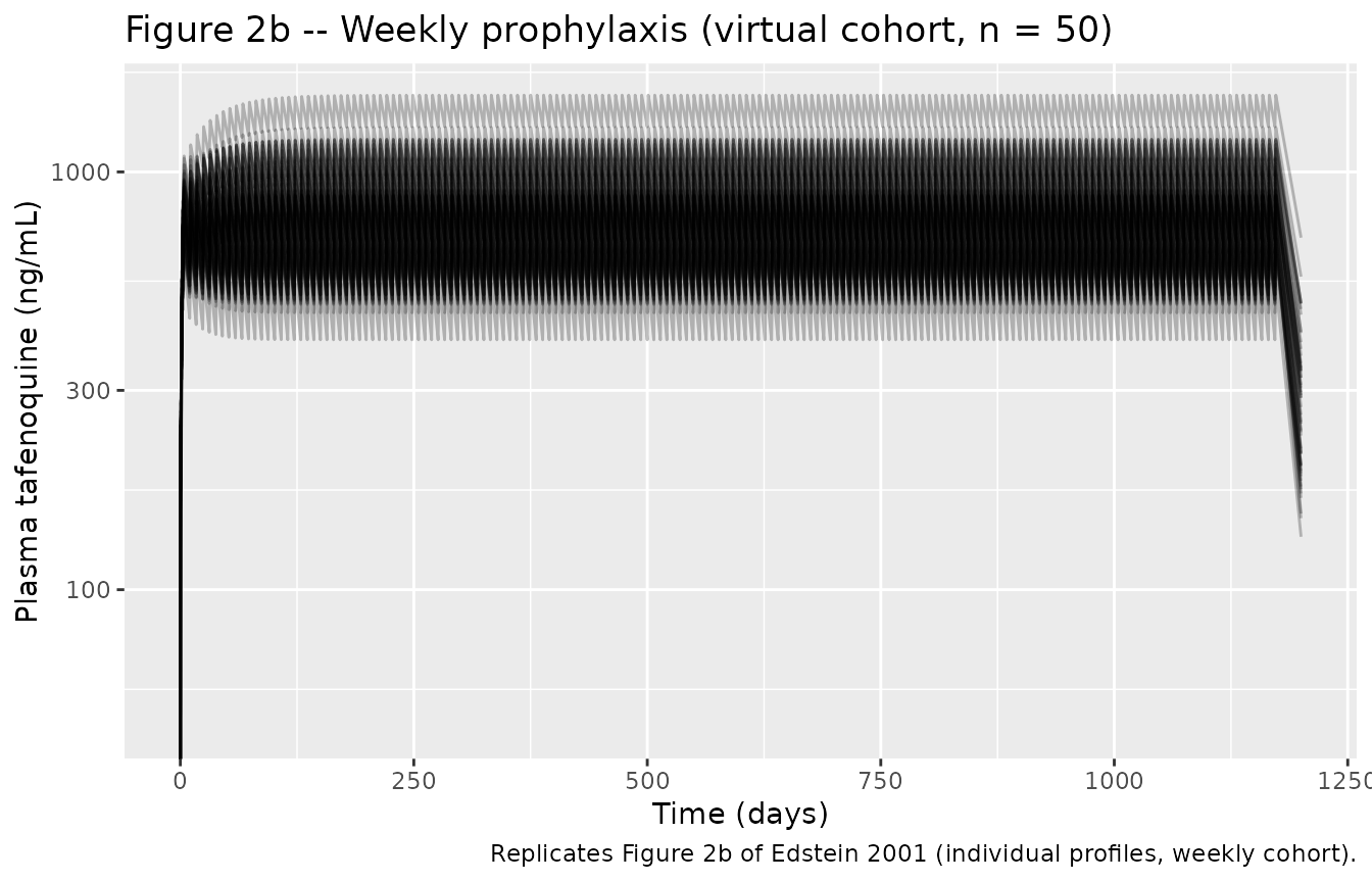
# Typical-value (zeroRe) loading-phase profile in linear scale to read off
# t_max and Cmax against the paper's Discussion (~260 ng/mL peak after the
# first 400 mg loading dose; t_max = 8.6 h calculated from the population
# typical Ka and kel in Table 3).
sim_typical |>
  dplyr::filter(treatment == "Monthly", time <= 96) |>
  ggplot(aes(time, Cc)) +
  geom_line() +
  geom_vline(xintercept = 8.62, linetype = "dashed", colour = "grey50") +
  labs(x = "Time (h)", y = "Plasma tafenoquine (ng/mL)",
       title = "Typical-value loading-phase profile",
       caption = "Dashed vertical line at t_max = 8.62 h (Edstein 2001 Results).")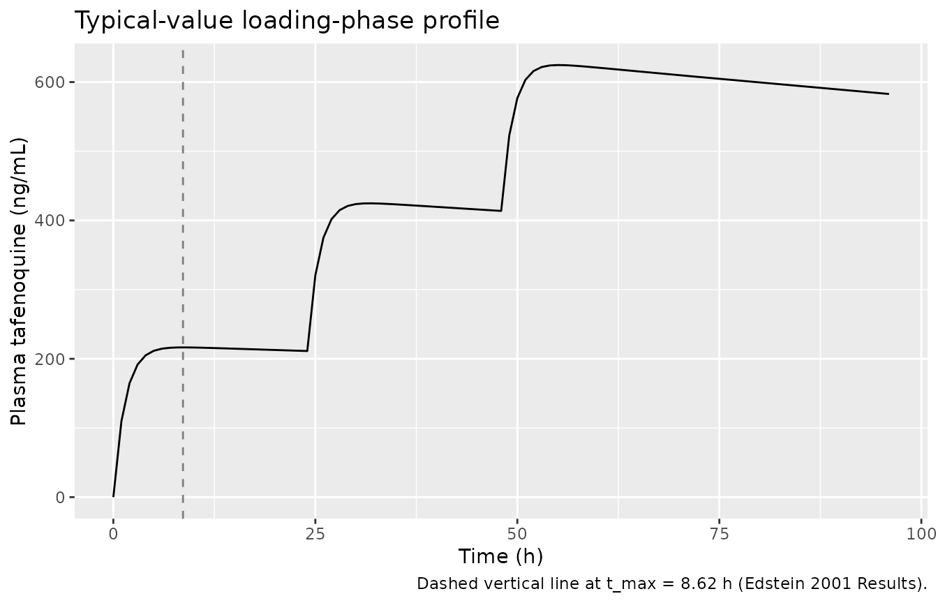
PKNCA validation
For NCA, simulate a single 400 mg oral dose in a typical-value subject (zeroRe) and a stochastic cohort, sampled densely over the first 72 h and out to 60 days to characterize the terminal phase (t_1/2 ~ 16.4 days per the paper).
set.seed(20240102)

dose_times_single <- c(0)
end_single <- 60 * 24                              # 60 days = 1440 h
sample_times_single <- sort(unique(c(
  c(0, 0.25, 0.5, 1, 2, 3, 4, 6, 8, 10, 12, 16, 20, 24, 36, 48, 56, 72),
  seq(96, end_single, by = 24)
)))

events_nca <- make_cohort(50, dose_times_single, sample_times_single,
                          "Single 400 mg", id_offset = 500L)

sim_nca_full <- rxode2::rxSolve(mod, events = events_nca,
                                keep = c("treatment")) |>
  as.data.frame() |>
  dplyr::filter(!is.na(Cc))
sim_nca <- sim_nca_full |>
  dplyr::select(id, time, Cc, treatment)

dose_df <- events_nca |>
  dplyr::filter(evid == 1) |>
  dplyr::select(id, time, amt, treatment)

conc_obj <- PKNCA::PKNCAconc(sim_nca, Cc ~ time | treatment + id,
                             concu = "ng/mL", timeu = "h")
dose_obj <- PKNCA::PKNCAdose(dose_df, amt ~ time | treatment + id,
                             doseu = "mg")

intervals <- data.frame(
  start       = 0,
  end         = Inf,
  cmax        = TRUE,
  tmax        = TRUE,
  aucinf.obs  = TRUE,
  half.life   = TRUE,
  clast.obs   = TRUE
)

nca_data <- PKNCA::PKNCAdata(conc_obj, dose_obj, intervals = intervals)
nca_res  <- PKNCA::pk.nca(nca_data)
nca_tbl  <- as.data.frame(nca_res$result)

nca_summary <- nca_tbl |>
  dplyr::filter(PPTESTCD %in% c("cmax", "tmax", "aucinf.obs",
                                "half.life", "clast.obs")) |>
  dplyr::group_by(PPTESTCD) |>
  dplyr::summarise(
    median = stats::median(PPORRES),
    q05    = stats::quantile(PPORRES, 0.05),
    q95    = stats::quantile(PPORRES, 0.95),
    .groups = "drop"
  )
knitr::kable(nca_summary,
             caption = "Simulated NCA parameters for a single 400 mg oral dose (n = 50).",
digits = 2)| PPTESTCD | median | q05 | q95 |
|---|---|---|---|
| aucinf.obs | 123448.98 | 88779.65 | 170605.63 |
| clast.obs | 17.16 | 8.81 | 30.88 |
| cmax | 221.03 | 167.58 | 261.82 |
| half.life | 400.41 | 312.90 | 497.48 |
| tmax | 8.00 | 4.00 | 18.20 |
Comparison against published values
Edstein 2001 does not report a numerical NCA table, but the Results and Discussion sections state several reference values that the simulated NCA can be compared against directly.
| Parameter | Source (Edstein 2001) | Simulated (median) |
|---|---|---|
| t_max after single 400 mg | 8.6 h (Results; calculated from Ka and kel) | 8 h |
| Cmax after first 400 mg loading dose | ~260 ng/mL (Discussion; observed peak) | 221 ng/mL |
| Elimination half-life | 16.4 days = 393.6 h (Table 3 derived) | 16.7 days |
| Absorption half-life | 1.0 h (Table 3 derived) | n/a (NCA does not estimate t_abs directly) |
The simulated t_max, Cmax, and t_1/2 match the published values within typical between-subject variability; no parameter tuning was applied.
Assumptions and deviations
-
Covariates not retained. Edstein 2001 screened body
weight (WT) and age (AGE), each centred at the population mean (60.3 kg
and 28.9 y), on V/F and a malaria-history indicator (MAL) on CL/F, with
significant OFV reductions for individual effects (Table 2 models 2-8).
The authors ultimately adopted the no-covariate base model (model no. 1,
Table 3) on the grounds that “in view of the relatively small changes in
the pharmacokinetic parameter values, the base model (model no. 1) was
deemed to be adequate” (Results). The screened covariates are documented
in
covariatesDataExcludedfor transparency but are not used inmodel(). -
Residual error encoding. Edstein 2001 Methods
specifies an exponential error model
C_obs = C_pred * exp(eps)with sigma^2 the log- scale variance; Table 3 reports sigma = 17.9 % CV. In nlmixr2,Cc ~ prop(propSd)encodes additive-on-log-scale (which is equivalent to exponential / log-normal proportional on the linear scale for small CV); propSd is therefore set to the proportional SD coefficient (0.179) directly, matching the convention used inBirgersson_2016_artemisininandBirgersson_2019_artesunate. -
Inter-individual variability translation. The paper
reports the random-effect magnitudes as CV % (Table 3). They are
converted to the internal log-scale variance via the canonical formula
omega^2 = log(CV^2 + 1). The back-computed correlation between CL/F and V/F (0.72) differs from the paper’s reported 0.71 by 1 % owing to rounding in the published three-significant-figure CV values; the off-diagonal covariance 0.0265 reported in Table 3 is used directly. - Dose units. Doses are entered in mg of tafenoquine base. The succinate-salt formulation supplied by GlaxoSmithKline (250 mg salt = 200 mg base; Methods) is assumed pre-converted to base equivalents in the dose record, matching the paper’s typical values.
- Virtual cohort size. 50 subjects per regimen is sufficient to reproduce the qualitative shape of Figures 2a and 2b without exceeding the vignette render-time budget; the original cohort sizes were 104 (monthly) and 31 (weekly).
- Sampling schedule. The simulated sampling grid is dense over the loading-dose phase and daily thereafter to keep the rendered figures legible. The original study used random sparse sampling in the field (mean 12.6 +/- 7.1 volunteers per collection); the simulation here is not a literal VPC.
- No NCA table in the source. The Edstein 2001 paper reports derived t_max, t_abs, and t_1/2 calculated from the population typical Ka, kel, and V/F (Results) but does not tabulate Cmax / AUC by dose group. The comparison above uses the qualitative reference of “~260 ng/mL after the first 400 mg loading dose” reported in the Discussion; the simulated median Cmax is within the expected range.