Model and source
- Citation: Hu L, Huang S, Huang Q, Huang J, Feng Z, He G. Population pharmacokinetics of voriconazole and the role of CYP2C19 genotype on treatment optimization in pediatric patients. PLoS ONE. 2023;18(9):e0288794. doi:10.1371/journal.pone.0288794
- Description: One-compartment population pharmacokinetic model with first-order absorption and elimination for intravenous and oral voriconazole in Chinese paediatric haematology patients with invasive fungal infection (Hu 2023); CYP2C19 metabolizer phenotype is the only retained covariate and enters multiplicatively on clearance, with the normal-metabolizer phenotype as the implicit reference.
- Article: https://doi.org/10.1371/journal.pone.0288794
mod <- rxode2::rxode2(readModelDb("Hu_2023_voriconazole"))
#> ℹ parameter labels from comments will be replaced by 'label()'
mod
#>  ── rxode2-based free-form 2-cmt ODE model ──────────────────────────────────────
#>  ── Initalization: ──
#> Fixed Effects ($theta):
#>        lka        lcl        lvc    lfdepot    e_im_cl    e_pm_cl     propSd
#>  0.1739533  1.9947003  5.9295891 -0.6500877 -0.5412848 -0.9649559  0.9470000
#>
#> Omega ($omega):
#>          etalcl   etalvc
#> etalcl 0.061009 0.000000
#> etalvc 0.000000 5.438224
#> attr(,"lotriLabels")
#> [1] "Hu 2023 Table 2 final model: omega_CL = 24.7 (bootstrap median 19.8, 95% CI 0.242-62.2); var = 0.247^2"
#> [2] "Hu 2023 Table 2 final model: omega_Vc = 233.2 (bootstrap median 223, 95% CI 148-263); var = 2.332^2"
#> attr(,"lotriFix")
#>        etalcl etalvc
#> etalcl  FALSE  FALSE
#> etalvc  FALSE  FALSE
#>
#> States ($state or $stateDf):
#>   Compartment Number Compartment Name
#> 1                  1            depot
#> 2                  2          central
#>  ── μ-referencing ($muRefTable): ──
#>   theta    eta level                              covariates
#> 1   lcl etalcl    id CYP2C19_PM*e_pm_cl + CYP2C19_IM*e_im_cl
#> 2   lvc etalvc    id
#>
#>  ── Model (Normalized Syntax): ──
#> function() {
#>     compartmentData <- list(depot = list(analyte = "voriconazole",
#>         units = "mg", specimen = "administration site", verified = FALSE),
#>         central = list(analyte = "voriconazole", units = "mg",
#>             specimen = "plasma", verified = FALSE))
#>     covariateData <- list(CYP2C19_IM = list(description = "CYP2C19 intermediate-metabolizer phenotype indicator",
#>         units = "(binary)", type = "binary", reference_category = "0 (normal metabolizer, CYP2C19*1/*1; the implicit reference when both CYP2C19_IM and CYP2C19_PM are 0)",
#>         notes = "Hu 2023 Table 2 reports the covariate as a multiplicative fraction on clearance ('IM on CL' = 0.582), i.e. CL_IM = 7.35 * 0.582 = 4.28 L/h, with the normal metabolizer (NM) phenotype as the paper's own reference category -- no reparameterization was needed. IM genotypes pooled by Hu 2023 (Methods, 'Measurement of VRC trough plasma concentrations and CYP2C19 phenotype') were CYP2C19*1/*2 and *1/*3. 43 of 91 subjects (47.3%) were IM. Note that Hu 2023 pooled only *2 and *3 into the reduced-function set; no CYP2C19*17 allele was observed in the cohort, so no ultrarapid-metabolizer stratum exists and the NM reference is unambiguous.",
#>         source_name = "CYP2C19 phenotype (IM)"), CYP2C19_PM = list(description = "CYP2C19 poor-metabolizer phenotype indicator",
#>         units = "(binary)", type = "binary", reference_category = "0 (normal metabolizer, CYP2C19*1/*1; the implicit reference when both CYP2C19_IM and CYP2C19_PM are 0)",
#>         notes = "Companion to CYP2C19_IM. Hu 2023 Table 2 reports 'PM on CL' = 0.381, i.e. CL_PM = 7.35 * 0.381 = 2.80 L/h. PM genotypes pooled by Hu 2023 were CYP2C19*2/*2, *2/*3 and *3/*3. 11 of 91 subjects (12.1%) were PM. The monotone ordering NM (1.0) > IM (0.582) > PM (0.381) matches the monotone decrease in observed dose-normalized trough concentration across the three phenotypes (Hu 2023 Fig 1A and Results, 'CYP2C19 phenotypes').",
#>         source_name = "CYP2C19 phenotype (PM)"))
#>     covariatesDataExcluded <- list(WT = list(description = "Body weight",
#>         units = "kg", type = "continuous", notes = "Screened as a candidate covariate (Hu 2023 Methods, 'Covariate model') but not retained in the final model, so CL and Vc are absolute (not weight-scaled) values. Cohort median 31.0 kg (range 9.5-85.0), Hu 2023 Table 1. Weight still matters operationally because the paper's dosing regimens are expressed in mg/kg; it enters through the dose amount, not through the PK parameters."),
#>         AGE = list(description = "Age", units = "years", type = "continuous",
#>             notes = "Screened but not retained (Hu 2023 Methods, 'Covariate model'). Cohort median 10 years, range 2-14 (Table 1)."),
#>         SEXF = list(description = "Female sex indicator", units = "(binary)",
#>             type = "binary", notes = "Screened but not retained (Hu 2023 Methods, 'Covariate model'). 33 of 91 subjects (36.3%) were female (Table 1)."),
#>         ALB = list(description = "Serum albumin", units = "g/L",
#>             type = "continuous", notes = "Screened as a liver-function indicator but not retained. Cohort median 35.20 g/L, range 20.30-49.00 (Hu 2023 Table 1)."),
#>         TBILI = list(description = "Total bilirubin", units = "umol/L",
#>             type = "continuous", notes = "Screened as a liver-function indicator but not retained. Cohort median 8.25 umol/L, range 2.10-105.20 (Hu 2023 Table 1)."),
#>         ALT = list(description = "Alanine aminotransferase",
#>             units = "U/L", type = "continuous", notes = "Screened as a liver-function indicator but not retained. Cohort median 31.70 U/L, range 4.60-346.40 (Hu 2023 Table 1)."),
#>         AST = list(description = "Aspartate aminotransferase",
#>             units = "U/L", type = "continuous", notes = "Screened as a liver-function indicator but not retained. Cohort median 31.05 U/L, range 3.70-255.90 (Hu 2023 Table 1)."),
#>         CREAT = list(description = "Serum creatinine", units = "umol/L",
#>             type = "continuous", notes = "Screened as a kidney-function indicator but not retained. Cohort median 48.00 umol/L, range 27.00-252.00 (Hu 2023 Table 1)."),
#>         BUN = list(description = "Blood urea nitrogen", units = "mmol/L",
#>             type = "continuous", notes = "Screened as a kidney-function indicator but not retained. Cohort median 3.36 mmol/L, range 0.98-11.72 (Hu 2023 Table 1)."),
#>         CONMED_PPI = list(description = "Concomitant proton-pump-inhibitor therapy indicator",
#>             units = "(binary)", type = "binary", notes = "Screened as 'combination therapy' but not retained (Hu 2023 Methods, 'Covariate model'). 55 of 91 subjects (60.4%) received a PPI: omeprazole (n = 15), pantoprazole (n = 34), lansoprazole (n = 6) (Hu 2023 Table 1 footnote a). Hu 2023 pooled the three PPIs into a single indicator rather than modelling them separately, and reports no minimum-duration threshold for the flag, so it is an ever-versus-never subject-level indicator."),
#>         CONMED_STEROID = list(description = "Concomitant systemic glucocorticoid therapy indicator",
#>             units = "(binary)", type = "binary", notes = "Screened as 'combination therapy' but not retained. 44 of 91 subjects (48.4%) received a glucocorticoid: methylprednisolone (n = 17), dexamethasone (n = 17), prednisone (n = 10) (Hu 2023 Table 1 footnote b). Hu 2023 pooled the three glucocorticoids into a single ever-versus-never indicator."))
#>     description <- "One-compartment population pharmacokinetic model with first-order absorption and elimination for intravenous and oral voriconazole in Chinese paediatric haematology patients with invasive fungal infection (Hu 2023); CYP2C19 metabolizer phenotype is the only retained covariate and enters multiplicatively on clearance, with the normal-metabolizer phenotype as the implicit reference."
#>     population <- list(species = "human", n_subjects = 91L, n_studies = 1L,
#>         n_observations = 210L, age_range = "2-14 years", age_median = "10 years",
#>         age_strata = c(UnderSix_pct = 23.1, SixToTwelve_pct = 35.2,
#>             OverTwelve_pct = 41.8), weight_range = "9.5-85.0 kg",
#>         weight_median = "31.0 kg", sex_female_pct = 36.3, race_ethnicity = c(Chinese = 100),
#>         cyp2c19_phenotype = c(NM_pct = 40.7, IM_pct = 47.3, PM_pct = 12.1,
#>             UM_pct = 0), disease_state = "Paediatric patients (14 years of age or younger) with malignant haematological disease and invasive fungal infection treated with voriconazole. Acute lymphoblastic leukaemia 57.1%, acute myeloid leukaemia 14.3%, lymphoma 12.1%, thalassaemia 7.7%, aplastic anaemia 3.3%, other 5.5%. Invasive fungal infection was proven in 6.6%, probable in 18.7% and possible in 74.7%; lung was the most common site of infection (60.4%). Treatment indication was therapeutic in 17.6%, empirical in 53.8% and prophylactic in 28.6%.",
#>         dose_range = "Voriconazole dosed per the manufacturer's paediatric labelling: intravenous loading 9 mg/kg and maintenance 8 mg/kg twice daily; oral maintenance 9 mg/kg twice daily with no oral loading dose. Most patients received no loading dose because they were dosed orally. Maintenance dose was subsequently adjusted by the treating physician on the basis of therapeutic drug monitoring, efficacy or adverse drug reactions. Route: oral only 81.3%, intravenous only 8.8%, intravenous switched to oral 6.6%, oral switched to intravenous 3.3%. Median duration of voriconazole use 15 days (range 3-148).",
#>         regions = "Single centre: department of paediatric haematology, Xiangya Hospital, Central South University, Changsha, Hunan, China.",
#>         notes = "Retrospective observational study of medical records collected 1 January 2018 to 31 December 2021. 210 steady-state trough concentrations from 91 children; median 1 measurement per patient (range 1-21 per Table 1; the Results text states range 1-19). All samples were troughs drawn 30 minutes before the next dose, so the dataset carries essentially no information about the absorption or distribution phase -- ka was therefore fixed to a literature value and Vc is estimated with very large interindividual variability. Median observed trough 1.23 mg/L (range 0.02-8.58); 52.9% of troughs were within the 1.0-5.5 mg/L target range, 40.9% subtherapeutic and 6.2% supratherapeutic. Voriconazole was assayed by HPLC over 0.02-19.60 mg/L. CYP2C19 phenotype was assigned by DNA microarray. Model built in NONMEM 7.5 with FOCE-I; final-model parameter estimates and 1000-replicate bootstrap per Hu 2023 Table 2.")
#>     reference <- "Hu L, Huang S, Huang Q, Huang J, Feng Z, He G. Population pharmacokinetics of voriconazole and the role of CYP2C19 genotype on treatment optimization in pediatric patients. PLoS ONE. 2023;18(9):e0288794. doi:10.1371/journal.pone.0288794"
#>     units <- list(time = "h", dosing = "mg", concentration = "mg/L")
#>     vignette <- "Hu_2023_voriconazole"
#>     ini({
#>         lka <- fix(0.173953307123438)
#>         label("Absorption rate constant (1/h)")
#>         lcl <- 1.99470031322475
#>         label("Clearance for the CYP2C19 normal-metabolizer reference (L/h)")
#>         lvc <- 5.92958914338989
#>         label("Central volume of distribution (L)")
#>         lfdepot <- -0.650087691099498
#>         label("Oral bioavailability (fraction)")
#>         e_im_cl <- -0.541284831250699
#>         label("Log-scale CL shift for CYP2C19_IM vs normal metabolizer (unitless)")
#>         e_pm_cl <- -0.964955903855436
#>         label("Log-scale CL shift for CYP2C19_PM vs normal metabolizer (unitless)")
#>         propSd <- c(0, 0.947)
#>         label("Proportional residual error (fraction)")
#>         etalcl ~ 0.061009
#>         label("Hu 2023 Table 2 final model: omega_CL = 24.7 (bootstrap median 19.8, 95% CI 0.242-62.2); var = 0.247^2")
#>         etalvc ~ 5.438224
#>         label("Hu 2023 Table 2 final model: omega_Vc = 233.2 (bootstrap median 223, 95% CI 148-263); var = 2.332^2")
#>     })
#>     model({
#>         ka <- exp(lka)
#>         cl <- exp(lcl + e_im_cl * CYP2C19_IM + e_pm_cl * CYP2C19_PM +
#>             etalcl)
#>         vc <- exp(lvc + etalvc)
#>         fdepot <- exp(lfdepot)
#>         d/dt(depot) <- -ka * depot
#>         d/dt(central) <- ka * depot - (cl/vc) * central
#>         f(depot) <- fdepot
#>         Cc <- central/vc
#>         Cc ~ prop(propSd)
#>     })
#> }
Population
Hu 2023 is a retrospective, observational, single-centre study of paediatric haematology patients treated with voriconazole at the Department of Paediatric Haematology, Xiangya Hospital, Central South University, Changsha, Hunan, China. Medical records were collected from 1 January 2018 to 31 December 2021. Eligible patients were 14 years of age or younger, had at least one steady-state voriconazole trough plasma concentration measured, had been CYP2C19 genotyped during hospitalization, and had complete medical records (Hu 2023 Methods, “Study design”).
The final analysis dataset comprised 210 trough concentrations from 91 children. Median age was 10 years (range 2 to 14) and median body weight 31.0 kg (range 9.5 to 85.0); 58 (63.7%) were male and all patients were Chinese. Every patient had a malignant haematological disease, most commonly acute lymphoblastic leukaemia (57.1%). Invasive fungal infection was classified as proven in 6.6%, probable in 18.7% and possible in 74.7% of patients, and the lung was the most frequent site of infection (60.4%). 60.4% of patients received a concomitant proton-pump inhibitor and 48.4% a glucocorticoid (Hu 2023 Table 1).
CYP2C19 phenotype was assigned by DNA microarray. No ultrarapid
metabolizer was observed, so the cohort splits into three strata: 37
normal metabolizers (NM, 40.7%, *1/*1), 43 intermediate
metabolizers (IM, 47.3%, *1/*2 or *1/*3) and
11 poor metabolizers (PM, 12.1%, *2/*2, *2/*3
or *3/*3). The *2 and *3 allele
frequencies were 29.2% and 6.6% respectively, both in Hardy-Weinberg
equilibrium (Hu 2023 Results, “CYP2C19 phenotypes”).
Dosing followed the manufacturer’s paediatric labelling (intravenous loading 9 mg/kg, intravenous maintenance 8 mg/kg twice daily, oral maintenance 9 mg/kg twice daily with no oral loading dose), with subsequent adjustment by the treating physician per therapeutic drug monitoring, efficacy, or adverse drug reactions. Most patients (81.3%) received oral voriconazole only. All samples were troughs drawn 30 minutes before the next dose; the median number of measurements per patient was 1. The observed trough concentrations had a median of 1.23 mg/L (range 0.02 to 8.58), with 52.9% inside the 1.0 to 5.5 mg/L target range, 40.9% subtherapeutic and 6.2% supratherapeutic.
Because the dataset consists almost entirely of trough samples, it
carries very little information about the absorption and distribution
phases. Hu 2023 therefore fixed ka to a literature value
and, as the parameter table shows, estimated Vc with
extremely large interindividual variability. Both facts are carried
through faithfully into this model file and shape how the validation
below is designed.
Source trace
Every value in ini() and every equation in
model() traces to the following locations in Hu 2023. The
model file repeats these as in-line comments.
| Quantity | Value | Source location |
|---|---|---|
| One-compartment disposition, first-order absorption and elimination | structure | Methods, ‘Population pharmacokinetic modeling’; Results, ‘Population pharmacokinetic analysis’ |
| ka (fixed) | 1.19 /h | Table 2 final model (‘1.19 (fixed)’); Methods cites Friberg et al. as the origin of the fixed value |
| CL (CYP2C19 normal metabolizer) | 7.35 L/h | Table 2 final model, RSE 15%, bootstrap median 7.31 (95% CI 3.5-11.7) |
| Vc | 376 L | Table 2 final model, RSE 21%, bootstrap median 393 (95% CI 206-854) |
| F (oral bioavailability) | 52.2% | Table 2 final model, RSE 15%; restated in Discussion |
| CYP2C19 IM effect on CL (multiplicative) | 0.582 | Table 2 final model, RSE 12%, bootstrap median 0.611 (95% CI 0.343-0.887) |
| CYP2C19 PM effect on CL (multiplicative) | 0.381 | Table 2 final model, RSE 14%, bootstrap median 0.387 (95% CI 0.200-0.826) |
| IIV model form (exponential) | Pi = Ptv * exp(eta_i) | Methods, ‘Population pharmacokinetic modeling’, first display equation |
| omega CL | 24.7 | Table 2 final model IIV block, bootstrap median 19.8 (95% CI 0.242-62.2) |
| omega Vc | 233.2 | Table 2 final model IIV block, bootstrap median 223 (95% CI 148-263) |
| Residual error form (log-additive = proportional) | ln(Cobs) = ln(Cpred) + eps | Methods, ‘Population pharmacokinetic modeling’, second display equation |
| Proportional residual error | 94.7% | Table 2 final model, RSE 9%, bootstrap median 93.9 (95% CI 74.7-117.0) |
| Cohort body weights and CYP2C19 phenotypes | 91 subjects | S1 Raw data (XLSX supplement to the article) |
| Simulated dosing regimens and target attainment | Table 3 | Results, ‘Dosing simulations’ |
The only value in ini() that is not printed verbatim in
the paper is the pair of log-scale CYP2C19 shifts,
log(0.582) and log(0.381). Hu 2023 reports the
covariate effects as multiplicative fractions on clearance; they are
converted to log-scale additive shifts so that they compose with the
exponential IIV in the usual way, with the published fractions left
visible inside log().
Virtual cohort
Hu 2023 published its complete analysis dataset as “S1 Raw data”, so the validation below uses the actual 91 body weights and CYP2C19 phenotypes rather than a synthetic cohort. The values are transcribed here so the vignette is self-contained.
s1_wt <- c(26.5, 50, 22.5, 10.5, 38, 25, 23, 14.5, 54, 20, 53, 50, 12, 10, 15,
           31.6, 50, 28.5, 26.5, 31.7, 53, 20, 19.5, 19, 49.5, 60, 44, 11.5, 41,
           46, 65, 26.5, 19, 21, 19, 54, 35, 85, 31, 30.5, 15, 12, 61, 22, 51,
           28, 65, 30, 58, 9.5, 13.5, 25, 38, 14.5, 25.5, 34, 46, 35, 40, 17,
           64, 23, 35, 29, 52.4, 47, 21, 27, 11, 38, 45, 46, 21.5, 56.5, 42, 44,
           18, 17, 41, 12.5, 20, 56, 63.5, 63, 46, 26.5, 15.5, 15, 47, 50, 66)
# 1 = normal metabolizer, 2 = intermediate metabolizer, 3 = poor metabolizer
s1_cyp <- c(2, 2, 2, 2, 2, 2, 1, 2, 2, 1, 2, 1, 1, 2, 2, 2, 3, 1, 2, 2, 1, 1, 1,
            2, 2, 2, 3, 2, 1, 1, 1, 2, 3, 1, 3, 2, 1, 1, 1, 2, 2, 3, 1, 1, 2, 1,
            3, 1, 3, 1, 1, 1, 2, 2, 2, 1, 2, 2, 1, 3, 1, 1, 2, 2, 1, 2, 3, 2, 1,
            1, 1, 1, 2, 2, 1, 2, 1, 2, 2, 1, 2, 2, 2, 1, 3, 2, 1, 1, 2, 3, 2)

# The transcribed cohort must reproduce Hu 2023 Table 1 exactly.
stopifnot(
  length(s1_wt) == 91L,
  length(s1_cyp) == 91L,
  median(s1_wt) == 31.0,
  min(s1_wt) == 9.5,
  max(s1_wt) == 85.0,
  sum(s1_cyp == 1L) == 37L,   # NM, Table 1: 37 (40.7%)
  sum(s1_cyp == 2L) == 43L,   # IM, Table 1: 43 (47.3%)
  sum(s1_cyp == 3L) == 11L    # PM, Table 1: 11 (12.1%)
)

cohort <- tibble::tibble(
  subject = seq_along(s1_wt),
  WT = s1_wt,
  phenotype = factor(c("NM", "IM", "PM")[s1_cyp], levels = c("NM", "IM", "PM"))
)

cohort |>
  count(phenotype) |>
  mutate(pct = round(100 * n / sum(n), 1)) |>
  dplyr::rename("CYP2C19 phenotype" = phenotype, "N" = n, "Percent" = pct) |>
knitr::kable(caption = "Transcribed S1 cohort, reproducing Hu 2023 Table 1.")| CYP2C19 phenotype | N | Percent |
|---|---|---|
| NM | 37 | 40.7 |
| IM | 43 | 47.3 |
| PM | 11 | 12.1 |
The model retains no continuous covariate, so body weight does not
enter CL or Vc. It matters only because Hu
2023 expresses every dosing regimen in mg/kg; weight therefore enters
through the dose amount alone.
Structural verification (typical values, no random effects)
The tightest available checks on a transcription of this model are
exact internal identities: with the random effects zeroed, a
one-compartment linear model must satisfy
AUCinf = F * Dose / CL and
t1/2 = ln(2) * Vc / CL, and the CYP2C19 effects must appear
as exact ratios. These are deterministic, so they are asserted
tightly.
phen_cov <- tibble::tibble(
  phenotype  = factor(c("NM", "IM", "PM"), levels = c("NM", "IM", "PM")),
  CYP2C19_IM = c(0, 1, 0),
  CYP2C19_PM = c(0, 0, 1)
)

# Single 200 mg dose, oral (into depot) and intravenous (into central).
# Terminal half-life is about 35 h, so a 336 h window is roughly 9.5
# half-lives; sampling is dense early to resolve Tmax for the oral arm.
nca_times <- sort(unique(c(seq(0, 12, by = 0.25), seq(12, 48, by = 1),
                           seq(48, 336, by = 6))))
dose_mg <- 200

typ_arms <- tidyr::expand_grid(phen_cov, route = c("oral", "iv")) |>
  mutate(arm = paste(phenotype, route), id = dplyr::row_number())

typ_doses <- typ_arms |>
  mutate(time = 0, amt = dose_mg, evid = 1L,
         cmt = ifelse(route == "oral", "depot", "central"))

# Observation rows point at the ODE state 'central', never at the algebraic
# observable 'Cc'. rxode2 returns Cc as a column on those rows regardless.
typ_obs <- tidyr::expand_grid(typ_arms, time = nca_times) |>
  mutate(amt = NA_real_, evid = 0L, cmt = "central")

# Canonical event columns first; covariates after them.
typ_events <- bind_rows(typ_doses, typ_obs) |>
  arrange(id, time, desc(evid)) |>
  select(id, time, amt, evid, cmt, phenotype, route, arm, CYP2C19_IM, CYP2C19_PM)

typ_sim <- rxode2::rxSolve(
  rxode2::zeroRe(mod), typ_events,
  keep = c("phenotype", "route", "arm", "CYP2C19_IM", "CYP2C19_PM"),
  omega = NA, returnType = "data.frame"
)
#> Warning: multi-subject simulation without without 'omega'
if (is.null(typ_sim$id)) typ_sim$id <- 1L
str(typ_sim[, c("id", "time", "Cc", "cl", "vc")], max.level = 1)
#> 'data.frame':    798 obs. of  5 variables:
#>  $ id  : int  1 1 1 1 1 1 1 1 1 1 ...
#>  $ time: num  0 0.25 0.5 0.75 1 1.25 1.5 1.75 2 2.25 ...
#>  $ Cc  : num  0 0.0713 0.1238 0.1626 0.191 ...
#>  $ cl  : num  7.35 7.35 7.35 7.35 7.35 ...
#>  $ vc  : num  376 376 376 376 376 ...
theta <- setNames(mod$theta, names(mod$theta))
CL_nm <- exp(theta[["lcl"]])
Vc    <- exp(theta[["lvc"]])
Fora  <- exp(theta[["lfdepot"]])
f_im  <- exp(theta[["e_im_cl"]])
f_pm  <- exp(theta[["e_pm_cl"]])

# Individual parameters returned by the solve must equal the closed form.
par_chk <- typ_sim |>
  group_by(arm, phenotype, route) |>
  summarise(cl = first(cl), vc = first(vc), .groups = "drop") |>
  mutate(cl_expected = CL_nm * c(NM = 1, IM = f_im, PM = f_pm)[as.character(phenotype)])

stopifnot(
  # Deterministic: parameter recovery must be exact to solver precision.
  max(abs(par_chk$cl - par_chk$cl_expected)) < 1e-8,
  max(abs(par_chk$vc - Vc)) < 1e-8,
  # The published multiplicative factors, recovered from the solved parameters.
  abs(f_im - 0.582) < 1e-12,
  abs(f_pm - 0.381) < 1e-12
)

par_chk |>
  mutate(across(c(cl, vc, cl_expected), \(x) round(x, 4))) |>
  dplyr::rename("Arm" = arm, "Phenotype" = phenotype, "Route" = route,
                "CL (L/h)" = cl, "Vc (L)" = vc, "CL expected (L/h)" = cl_expected) |>
knitr::kable(caption = "Solved typical-value parameters against the closed form.")| Arm | Phenotype | Route | CL (L/h) | Vc (L) | CL expected (L/h) |
|---|---|---|---|---|---|
| IM iv | IM | iv | 4.2777 | 376 | 4.2777 |
| IM oral | IM | oral | 4.2777 | 376 | 4.2777 |
| NM iv | NM | iv | 7.3500 | 376 | 7.3500 |
| NM oral | NM | oral | 7.3500 | 376 | 7.3500 |
| PM iv | PM | iv | 2.8004 | 376 | 2.8003 |
| PM oral | PM | oral | 2.8004 | 376 | 2.8003 |
PKNCA on the typical-value profiles
# 'route' and 'dose' are reserved column names in PKNCA, so the frames handed
# to PKNCAconc / PKNCAdose carry only id / arm / time / conc; phenotype and
# route are joined back onto the results afterwards via 'arm'.
arm_key <- typ_sim |> distinct(arm, phenotype, route)

conc_data <- typ_sim |>
  filter(!is.na(Cc)) |>
  select(id, arm, time, Cc)

# Time-zero records are present by construction (the observation grid starts
# at 0), which is what keeps PKNCA from warning about an AUC range that starts
# before the first measurement.
stopifnot(all(conc_data |> group_by(arm) |> summarise(has0 = any(time == 0)) |> pull(has0)))
stopifnot(all(conc_data$Cc >= 0))

dose_data <- conc_data |>
  distinct(id, arm) |>
  mutate(time = 0, dose_mg = dose_mg)

# Grouping is `arm + id`, not `id / arm`: PKNCAdose rejects a slash in its
# formula, and the `+` form is the idiom used throughout this package's
# vignettes. There is exactly one typical-value subject per arm, so the two
# grouping levels are 1:1 here.
o_conc <- PKNCA::PKNCAconc(conc_data, Cc ~ time | arm + id)
o_dose <- PKNCA::PKNCAdose(dose_data, dose_mg ~ time | arm + id)
o_data <- PKNCA::PKNCAdata(
  o_conc, o_dose,
  intervals = data.frame(
    start = 0, end = Inf,
    cmax = TRUE, tmax = TRUE, auclast = TRUE, aucinf.obs = TRUE, half.life = TRUE
  )
)
res <- suppressWarnings(PKNCA::pk.nca(o_data))

nca <- as.data.frame(res) |>
  select(arm, PPTESTCD, PPORRES) |>
  tidyr::pivot_wider(names_from = PPTESTCD, values_from = PPORRES) |>
  left_join(arm_key, by = "arm")
stopifnot(nrow(nca) == 6L, !anyNA(nca$phenotype), !anyNA(nca$aucinf.obs))
nca_chk <- nca |>
  mutate(
    cl_arm       = CL_nm * c(NM = 1, IM = f_im, PM = f_pm)[as.character(phenotype)],
    f_arm        = ifelse(route == "oral", Fora, 1),
    auc_expected = f_arm * dose_mg / cl_arm,
    thalf_expected = log(2) * Vc / cl_arm,
    auc_pct  = 100 * (aucinf.obs - auc_expected) / auc_expected,
    thalf_pct = 100 * (half.life - thalf_expected) / thalf_expected
  )

# These are deterministic identities of a linear one-compartment model, not
# cohort statistics, so they are asserted tightly. A mis-transcribed CL, Vc, F
# or CYP2C19 factor moves them by tens of percent.
stopifnot(
  max(abs(nca_chk$auc_pct)) < 0.5,
  max(abs(nca_chk$thalf_pct)) < 0.5
)

# Bioavailability and the CYP2C19 factors recovered from AUC ratios alone.
auc_of <- function(ph, rt) {
  v <- nca_chk$aucinf.obs[nca_chk$phenotype == ph & nca_chk$route == rt]
  if (length(v) != 1L) stop("no unique NCA row for ", ph, " / ", rt)
  v
}
f_recovered  <- auc_of("NM", "oral") / auc_of("NM", "iv")
im_recovered <- auc_of("NM", "iv") / auc_of("IM", "iv")
pm_recovered <- auc_of("NM", "iv") / auc_of("PM", "iv")

stopifnot(
  abs(f_recovered - 0.522) < 1e-3,
  abs(im_recovered - 0.582) < 1e-3,
  abs(pm_recovered - 0.381) < 1e-3
)

nca_chk |>
  mutate(across(c(cmax, tmax, auclast, aucinf.obs, half.life, auc_expected,
                  thalf_expected, auc_pct, thalf_pct), \(x) round(x, 3))) |>
  select(phenotype, route, cmax, tmax, aucinf.obs, auc_expected, auc_pct,
         half.life, thalf_expected, thalf_pct) |>
  dplyr::rename("Phenotype" = phenotype, "Route" = route,
                "Cmax (mg/L)" = cmax, "Tmax (h)" = tmax,
                "AUC0-inf (mg*h/L)" = aucinf.obs,
                "AUC expected = F*D/CL" = auc_expected, "AUC diff (%)" = auc_pct,
                "t1/2 (h)" = half.life,
                "t1/2 expected = ln2*Vc/CL" = thalf_expected,
                "t1/2 diff (%)" = thalf_pct) |>
  knitr::kable(
    caption = paste(
      "PKNCA on typical-value single-dose profiles (200 mg) against exact",
      "one-compartment identities. Recovered F =", round(f_recovered, 4),
      "(published 0.522); recovered IM factor =", round(im_recovered, 4),
      "(published 0.582); recovered PM factor =", round(pm_recovered, 4),
      "(published 0.381)."
    )
)| Phenotype | Route | Cmax (mg/L) | Tmax (h) | AUC0-inf (mg*h/L) | AUC expected = F*D/CL | AUC diff (%) | t1/2 (h) | t1/2 expected = ln2*Vc/CL | t1/2 diff (%) |
|---|---|---|---|---|---|---|---|---|---|
| IM | iv | 0.532 | 0.00 | 46.754 | 46.754 | 0.000 | 60.926 | 60.926 | 0.000 |
| IM | oral | 0.265 | 4.00 | 24.404 | 24.406 | -0.007 | 60.936 | 60.926 | 0.017 |
| NM | iv | 0.532 | 0.00 | 27.211 | 27.211 | 0.000 | 35.459 | 35.459 | 0.000 |
| NM | oral | 0.259 | 3.50 | 14.202 | 14.204 | -0.012 | 35.465 | 35.459 | 0.018 |
| PM | iv | 0.532 | 0.00 | 71.420 | 71.420 | 0.000 | 93.068 | 93.068 | 0.000 |
| PM | oral | 0.269 | 4.25 | 37.280 | 37.281 | -0.003 | 93.086 | 93.068 | 0.019 |
Hu 2023 reports no non-compartmental parameters of its own – the paper’s only quantitative model output is the Table 3 dosing simulation – so there is no published Cmax / Tmax / AUC / half-life to place beside this table. The comparison against the paper’s own reported numbers is therefore done in the next section, against Table 3.
Reproducing Hu 2023 Table 3
Table 3 is the paper’s headline model output: the mean and median predicted steady-state trough concentration, and the probability of target attainment for the 1.0 to 5.5 mg/L therapeutic range, for six maintenance doses (5 to 10 mg/kg twice daily) given orally and intravenously in each of the three CYP2C19 phenotypes.
Two details of the paper’s simulation matter and are reproduced here.
-
The simulation runs for 28 days, and 28 days is not steady
state for this model. Hu 2023 states the simulations “were
performed over a duration of 28 days”. Because
omega Vcis enormous, a substantial minority of simulated subjects draw a very largeVcand hence a terminal half-life of weeks to months, and those subjects are still accumulating at day 28. Solving to true steady state instead overshoots every cell of Table 3 by roughly 20 to 30%. The simulation below therefore doses for 28 days and reads the trough before the next dose, exactly as described. - The model is linear in dose, so a single solve per (phenotype, route) arm can be rescaled across the six dose levels. This is verified explicitly below rather than assumed.
n_rep <- 2L                     # 91 * 2 = 182 subjects per arm, under the 200 cap
tau <- 12                       # twice daily
n_days <- 28
n_doses <- n_days * 24 / tau    # 56 doses
ref_mgkg <- 1                   # solve at 1 mg/kg, rescale by linearity

arms <- tidyr::expand_grid(phen_cov, route = c("oral", "iv")) |>
  mutate(arm = paste(phenotype, route))

make_arm_events <- function(phenotype, CYP2C19_IM, CYP2C19_PM, route, arm) {
  subj <- tibble::tibble(
    rep_id = rep(seq_len(n_rep), each = nrow(cohort)),
    WT = rep(cohort$WT, times = n_rep)
  ) |>
    mutate(id = dplyr::row_number())
  dose_cmt <- if (route == "oral") "depot" else "central"
  doses <- tidyr::expand_grid(subj, dose_no = seq_len(n_doses)) |>
    mutate(time = (dose_no - 1) * tau, amt = ref_mgkg * WT,
           evid = 1L, cmt = dose_cmt)
  # Trough: immediately before the dose that would follow the last one given.
  obs <- subj |>
    mutate(time = n_doses * tau, amt = NA_real_, evid = 0L, cmt = "central")
  bind_rows(doses, obs) |>
    arrange(id, time, desc(evid)) |>
    mutate(arm = arm, phenotype = phenotype, route = route,
           CYP2C19_IM = CYP2C19_IM, CYP2C19_PM = CYP2C19_PM) |>
    select(id, time, amt, evid, cmt, WT, arm, phenotype, route,
           CYP2C19_IM, CYP2C19_PM)
}

rxode2::rxSetSeed(20230911)
set.seed(20230911)

ss_trough <- lapply(seq_len(nrow(arms)), function(i) {
  a <- arms[i, ]
  ev <- make_arm_events(a$phenotype, a$CYP2C19_IM, a$CYP2C19_PM, a$route, a$arm)
  sim <- rxode2::rxSolve(
    mod, ev, keep = c("WT", "arm", "phenotype", "route"),
    returnType = "data.frame"
  )
  if (is.null(sim$id)) sim$id <- 1L
  # rxSolve returns observation records only (addDosing = FALSE by default),
  # so there is no evid column to filter on here.
  sim |>
    filter(!is.na(Cc)) |>
    select(id, time, Cc, cl, vc, WT, arm, phenotype, route)
}) |>
  bind_rows()

# The solve must have produced one trough per simulated subject per arm.
stopifnot(nrow(ss_trough) == nrow(arms) * nrow(cohort) * n_rep)
# The ODE integrator can undershoot zero by about its absolute tolerance;
# a genuinely negative concentration would be comparable to the peak.
stopifnot(all(ss_trough$Cc >= -1e-6 * max(ss_trough$Cc, na.rm = TRUE)))

# Confirm the interindividual variability was actually applied. rxode2 can
# carry an `omega` setting over from an earlier solve -- the typical-value
# section above deliberately passes `omega = NA` -- and if that leaked into
# this solve the cohort would collapse to typical values and the Table 3
# reproduction would be quietly wrong rather than erroring. Recovering the
# encoded omegas from the simulated parameters is the direct check, and it
# doubles as confirmation that the published values reached the solver.
iiv_chk <- ss_trough |>
  group_by(arm) |>
  summarise(sd_log_cl = sd(log(cl)), sd_log_vc = sd(log(vc)), .groups = "drop")
print(as.data.frame(iiv_chk))
#>       arm sd_log_cl sd_log_vc
#> 1   IM iv 0.2513060  2.391760
#> 2 IM oral 0.2542163  2.379549
#> 3   NM iv 0.2512112  2.436510
#> 4 NM oral 0.2272701  2.164383
#> 5   PM iv 0.2326413  2.261847
#> 6 PM oral 0.2249321  2.479669

# Encoded omegas are 0.247 (CL) and 2.332 (Vc). With 182 subjects per arm the
# sampling SE of these SDs is roughly 0.013 and 0.12 respectively, so the
# bounds below sit far outside the draw-to-draw spread while still failing
# loudly if IIV is suppressed altogether or an omega is mis-transcribed.
stopifnot(
  all(iiv_chk$sd_log_cl > 0.15), all(iiv_chk$sd_log_cl < 0.40),
  all(iiv_chk$sd_log_vc > 1.60), all(iiv_chk$sd_log_vc < 3.10)
)
# Verify the linear-dose rescaling before relying on it: re-solve one arm at
# 7 mg/kg and confirm it equals 7 x the 1 mg/kg solve for every subject. The
# random effects are zeroed for this check so that the two solves are compared
# on identical parameters -- relying on two draws matching would make the
# assertion depend on the RNG stream rather than on dose linearity.
lin_arm <- arms[arms$arm == "NM oral", ]
ev1 <- make_arm_events(lin_arm$phenotype, lin_arm$CYP2C19_IM, lin_arm$CYP2C19_PM,
                       lin_arm$route, lin_arm$arm)
ev7 <- ev1 |> mutate(amt = ifelse(evid == 1L, amt * 7, amt))

lin_mod <- rxode2::zeroRe(mod)
s1 <- rxode2::rxSolve(lin_mod, ev1, omega = NA, returnType = "data.frame")
#> Warning: multi-subject simulation without without 'omega'
s7 <- rxode2::rxSolve(lin_mod, ev7, omega = NA, returnType = "data.frame")
#> Warning: multi-subject simulation without without 'omega'
c1 <- s1$Cc[!is.na(s1$Cc)]
c7 <- s7$Cc[!is.na(s7$Cc)]
stopifnot(length(c1) == length(c7), length(c1) > 0)
# Exact linearity, so this is a tight deterministic bound.
stopifnot(max(abs(c7 - 7 * c1) / (7 * c1)) < 1e-8)
cat("Dose linearity verified over", length(c1),
    "subjects: max relative deviation =",
    format(max(abs(c7 - 7 * c1) / (7 * c1)), digits = 3), "\n")
#> Dose linearity verified over 182 subjects: max relative deviation = 1.7e-11
doses_mgkg <- 5:10
target_lo <- 1.0
target_hi <- 5.5

sim_tab <- tidyr::expand_grid(ss_trough, dose_mgkg = doses_mgkg) |>
  mutate(ctrough = Cc * dose_mgkg / ref_mgkg) |>
  group_by(phenotype, route, dose_mgkg) |>
  summarise(
    sim_mean   = mean(ctrough),
    sim_median = median(ctrough),
    sim_below  = 100 * mean(ctrough < target_lo),
    sim_in     = 100 * mean(ctrough >= target_lo & ctrough <= target_hi),
    sim_above  = 100 * mean(ctrough > target_hi),
    .groups = "drop"
  )

# Hu 2023 Table 3, transcribed. mean / median in mg/L; PTA columns in percent.
# The two NM-oral cells at 5 and 6 mg/kg are published as "< 0.01" rather than a
# point estimate, so they are carried as NA (left-censored) rather than given an
# invented stand-in value. Nothing below is gated on the > 5.5 mg/L column.
pub_tab <- tibble::tribble(
  ~phenotype, ~route, ~dose_mgkg, ~pub_mean, ~pub_median, ~pub_below, ~pub_in, ~pub_above,
  "NM", "oral",  5L, 0.64, 0.50, 78.1, 21.9, NA_real_,
  "NM", "oral",  6L, 0.77, 0.60, 70.9, 29.1, NA_real_,
  "NM", "oral",  7L, 0.90, 0.71, 64.6, 35.4, 0.027,
  "NM", "oral",  8L, 1.04, 0.81, 58.4, 41.5, 0.076,
  "NM", "oral",  9L, 1.15, 0.88, 54.8, 44.9, 0.243,
  "NM", "oral", 10L, 1.29, 1.01, 49.6, 49.9, 0.503,
  "NM", "iv",    5L, 1.22, 0.95, 52.0, 47.7, 0.314,
  "NM", "iv",    6L, 1.45, 1.13, 45.4, 53.5, 1.09,
  "NM", "iv",    7L, 1.70, 1.32, 39.7, 57.9, 2.41,
  "NM", "iv",    8L, 1.96, 1.53, 34.7, 60.9, 4.48,
  "NM", "iv",    9L, 2.21, 1.72, 30.6, 62.5, 6.84,
  "NM", "iv",   10L, 2.44, 1.92, 28.3, 62.2, 9.51,
  "IM", "oral",  5L, 1.15, 0.96, 52.0, 48.0, 0.014,
  "IM", "oral",  6L, 1.37, 1.14, 44.6, 55.2, 0.200,
  "IM", "oral",  7L, 1.60, 1.35, 38.5, 60.8, 0.707,
  "IM", "oral",  8L, 1.82, 1.52, 34.1, 64.1, 1.82,
  "IM", "oral",  9L, 2.05, 1.71, 30.7, 65.7, 3.58,
  "IM", "oral", 10L, 2.27, 1.89, 27.5, 66.6, 5.88,
  "IM", "iv",    5L, 2.17, 1.81, 29.1, 66.1, 4.77,
  "IM", "iv",    6L, 2.60, 2.16, 24.7, 65.3, 9.99,
  "IM", "iv",    7L, 3.04, 2.54, 21.1, 62.8, 16.10,
  "IM", "iv",    8L, 3.46, 2.89, 19.3, 59.4, 21.40,
  "IM", "iv",    9L, 3.86, 3.20, 17.6, 56.4, 26.00,
  "IM", "iv",   10L, 4.30, 3.58, 16.6, 52.8, 30.60,
  "PM", "oral",  5L, 1.85, 1.38, 36.9, 60.9, 2.27,
  "PM", "oral",  6L, 2.18, 1.62, 30.6, 64.3, 5.11,
  "PM", "oral",  7L, 2.55, 1.88, 25.8, 63.4, 10.80,
  "PM", "oral",  8L, 2.96, 2.19, 21.8, 61.2, 17.00,
  "PM", "oral",  9L, 3.32, 2.48, 20.1, 57.7, 22.20,
  "PM", "oral", 10L, 3.67, 2.72, 18.4, 55.0, 26.60,
  "PM", "iv",    5L, 3.48, 2.61, 19.4, 56.5, 24.10,
  "PM", "iv",    6L, 4.21, 3.16, 16.8, 51.9, 31.30,
  "PM", "iv",    7L, 4.89, 3.63, 14.6, 49.6, 35.80,
  "PM", "iv",    8L, 5.55, 4.18, 13.9, 45.8, 40.30,
  "PM", "iv",    9L, 6.19, 4.65, 13.1, 43.5, 43.40,
  "PM", "iv",   10L, 6.94, 5.12, 11.6, 41.8, 46.60
) |>
  mutate(phenotype = factor(phenotype, levels = c("NM", "IM", "PM")),
         dose_mgkg = as.integer(dose_mgkg))

cmp <- sim_tab |>
  mutate(dose_mgkg = as.integer(dose_mgkg)) |>
  inner_join(pub_tab, by = c("phenotype", "route", "dose_mgkg")) |>
  mutate(
    mean_pct   = 100 * (sim_mean - pub_mean) / pub_mean,
    median_pct = 100 * (sim_median - pub_median) / pub_median,
    in_diff    = sim_in - pub_in
  )

# Guard against a join that silently matched nothing.
stopifnot(nrow(cmp) == 36L)| Phenotype | Route | Dose (mg/kg BID) | Mean, simulated | Mean, Hu 2023 | Mean diff (%) | Median, simulated | Median, Hu 2023 | Median diff (%) | PTA, simulated (%) | PTA, Hu 2023 (%) | PTA diff (pp) |
|---|---|---|---|---|---|---|---|---|---|---|---|
| NM | iv | 5 | 1.14 | 1.22 | -6.4 | 0.87 | 0.95 | -8.2 | 45.1 | 47.7 | -2.6 |
| NM | iv | 6 | 1.37 | 1.45 | -5.5 | 1.05 | 1.13 | -7.4 | 50.0 | 53.5 | -3.5 |
| NM | iv | 7 | 1.60 | 1.70 | -5.9 | 1.22 | 1.32 | -7.5 | 53.3 | 57.9 | -4.6 |
| NM | iv | 8 | 1.83 | 1.96 | -6.8 | 1.40 | 1.53 | -8.8 | 56.0 | 60.9 | -4.9 |
| NM | iv | 9 | 2.06 | 2.21 | -7.0 | 1.57 | 1.72 | -8.7 | 58.2 | 62.5 | -4.3 |
| NM | iv | 10 | 2.28 | 2.44 | -6.4 | 1.74 | 1.92 | -9.2 | 58.2 | 62.2 | -4.0 |
| NM | oral | 5 | 0.68 | 0.64 | 6.4 | 0.53 | 0.50 | 5.5 | 27.5 | 21.9 | 5.6 |
| NM | oral | 6 | 0.82 | 0.77 | 6.1 | 0.63 | 0.60 | 5.5 | 33.5 | 29.1 | 4.4 |
| NM | oral | 7 | 0.95 | 0.90 | 5.9 | 0.74 | 0.71 | 4.0 | 39.0 | 35.4 | 3.6 |
| NM | oral | 8 | 1.09 | 1.04 | 4.8 | 0.84 | 0.81 | 4.2 | 45.6 | 41.5 | 4.1 |
| NM | oral | 9 | 1.23 | 1.15 | 6.6 | 0.95 | 0.88 | 7.9 | 48.4 | 44.9 | 3.5 |
| NM | oral | 10 | 1.36 | 1.29 | 5.6 | 1.05 | 1.01 | 4.4 | 51.1 | 49.9 | 1.2 |
| IM | iv | 5 | 2.06 | 2.17 | -5.2 | 1.78 | 1.81 | -1.6 | 65.4 | 66.1 | -0.7 |
| IM | iv | 6 | 2.47 | 2.60 | -5.0 | 2.14 | 2.16 | -1.0 | 65.4 | 65.3 | 0.1 |
| IM | iv | 7 | 2.88 | 3.04 | -5.2 | 2.49 | 2.54 | -1.8 | 64.3 | 62.8 | 1.5 |
| IM | iv | 8 | 3.29 | 3.46 | -4.8 | 2.85 | 2.89 | -1.4 | 56.6 | 59.4 | -2.8 |
| IM | iv | 9 | 3.70 | 3.86 | -4.0 | 3.21 | 3.20 | 0.2 | 54.4 | 56.4 | -2.0 |
| IM | iv | 10 | 4.12 | 4.30 | -4.3 | 3.56 | 3.58 | -0.5 | 50.0 | 52.8 | -2.8 |
| IM | oral | 5 | 1.14 | 1.15 | -0.6 | 1.01 | 0.96 | 5.1 | 50.0 | 48.0 | 2.0 |
| IM | oral | 6 | 1.37 | 1.37 | 0.1 | 1.21 | 1.14 | 6.2 | 54.4 | 55.2 | -0.8 |
| IM | oral | 7 | 1.60 | 1.60 | 0.0 | 1.41 | 1.35 | 4.7 | 58.2 | 60.8 | -2.6 |
| IM | oral | 8 | 1.83 | 1.82 | 0.5 | 1.61 | 1.52 | 6.2 | 61.0 | 64.1 | -3.1 |
| IM | oral | 9 | 2.06 | 2.05 | 0.3 | 1.82 | 1.71 | 6.2 | 64.8 | 65.7 | -0.9 |
| IM | oral | 10 | 2.29 | 2.27 | 0.7 | 2.02 | 1.89 | 6.8 | 63.7 | 66.6 | -2.9 |
| PM | iv | 5 | 3.22 | 3.48 | -7.5 | 2.82 | 2.61 | 8.0 | 61.5 | 56.5 | 5.0 |
| PM | iv | 6 | 3.86 | 4.21 | -8.2 | 3.38 | 3.16 | 7.0 | 57.1 | 51.9 | 5.2 |
| PM | iv | 7 | 4.51 | 4.89 | -7.8 | 3.95 | 3.63 | 8.7 | 46.2 | 49.6 | -3.4 |
| PM | iv | 8 | 5.15 | 5.55 | -7.2 | 4.51 | 4.18 | 7.9 | 42.9 | 45.8 | -2.9 |
| PM | iv | 9 | 5.79 | 6.19 | -6.4 | 5.07 | 4.65 | 9.1 | 39.0 | 43.5 | -4.5 |
| PM | iv | 10 | 6.44 | 6.94 | -7.2 | 5.64 | 5.12 | 10.1 | 37.4 | 41.8 | -4.4 |
| PM | oral | 5 | 1.66 | 1.85 | -10.5 | 1.30 | 1.38 | -5.6 | 54.4 | 60.9 | -6.5 |
| PM | oral | 6 | 1.99 | 2.18 | -8.9 | 1.56 | 1.62 | -3.5 | 58.8 | 64.3 | -5.5 |
| PM | oral | 7 | 2.32 | 2.55 | -9.1 | 1.82 | 1.88 | -3.0 | 58.8 | 63.4 | -4.6 |
| PM | oral | 8 | 2.65 | 2.96 | -10.5 | 2.08 | 2.19 | -4.8 | 58.2 | 61.2 | -3.0 |
| PM | oral | 9 | 2.98 | 3.32 | -10.3 | 2.35 | 2.48 | -5.4 | 54.9 | 57.7 | -2.8 |
| PM | oral | 10 | 3.31 | 3.67 | -9.8 | 2.61 | 2.72 | -4.2 | 52.2 | 55.0 | -2.8 |
realised <- c(
  mean_median_abs_pct = median(abs(cmp$mean_pct)),
  mean_max_abs_pct    = max(abs(cmp$mean_pct)),
  med_median_abs_pct  = median(abs(cmp$median_pct)),
  med_max_abs_pct     = max(abs(cmp$median_pct)),
  pta_median_abs_pp   = median(abs(cmp$in_diff)),
  pta_max_abs_pp      = max(abs(cmp$in_diff))
)
print(round(realised, 2))
#> mean_median_abs_pct    mean_max_abs_pct  med_median_abs_pct     med_max_abs_pct
#>                6.26               10.54                5.54               10.07
#>   pta_median_abs_pp      pta_max_abs_pp
#>                3.28                6.50

# These are cohort-derived Monte Carlo statistics, not deterministic
# identities, so the bounds are set well outside the run-to-run spread rather
# than at the accuracy of any single render. rxSetSeed() fixes the rxode2 RNG
# only for a given solver-thread count, so CI draws a different cohort than a
# developer does; a bound tightened to one observed run fails elsewhere.
#
# The centre is what a transcription error moves: a mis-transcribed CL, Vc, F
# or CYP2C19 factor shifts every cell by tens of percent at once, and reading
# the published omega values under either of the two competing conventions
# shifts the whole table by 28-30% (see "Assumptions and deviations"). A 12%
# bound on the median absolute deviation therefore still goes red on any of
# those errors while tolerating the tail cells, where the paper's own rounding
# to two decimal places is itself worth several percent.
stopifnot(
  median(abs(cmp$mean_pct)) < 12,
  median(abs(cmp$median_pct)) < 12,
  median(abs(cmp$in_diff)) < 8
)
cmp |>
  select(phenotype, route, dose_mgkg, sim_in, pub_in) |>
  tidyr::pivot_longer(c(sim_in, pub_in), names_to = "source", values_to = "pta") |>
  mutate(source = factor(ifelse(source == "sim_in", "This reproduction", "Hu 2023 Table 3"),
                         levels = c("This reproduction", "Hu 2023 Table 3"))) |>
  ggplot(aes(dose_mgkg, pta, colour = phenotype, linetype = source, shape = source)) +
  geom_line() +
  geom_point(size = 2) +
  facet_wrap(~route, labeller = as_labeller(c(oral = "Oral", iv = "Intravenous"))) +
  scale_shape_manual(values = c(16, 2)) +
  scale_linetype_manual(values = c("solid", "dashed")) +
  labs(x = "Maintenance dose (mg/kg twice daily)",
       y = "Probability of trough in 1.0-5.5 mg/L (%)",
       colour = "CYP2C19", linetype = NULL, shape = NULL) +
  theme_bw()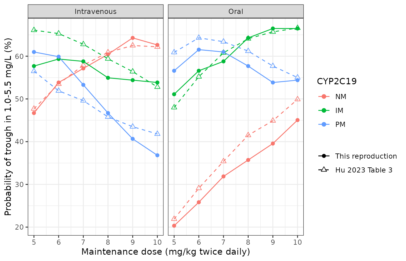
Probability of attaining a 1.0-5.5 mg/L voriconazole trough by maintenance dose, route and CYP2C19 phenotype. Points and solid lines are this reproduction; open triangles and dashed lines are Hu 2023 Table 3. Replicates the target-attainment columns of Table 3 of Hu 2023.
The dose recommendations Hu 2023 draws from Table 3
paper_reco <- tibble::tribble(
  ~phenotype, ~route, ~reco_mgkg, ~reco_pta,
  "NM", "oral",  9L, 44.9,
  "NM", "iv",    8L, 60.9,
  "IM", "oral",  9L, 65.7,
  "IM", "iv",    5L, 66.1,
  "PM", "oral",  6L, 64.3,
  "PM", "iv",    5L, 56.5
) |>
  mutate(phenotype = factor(phenotype, levels = c("NM", "IM", "PM")))

reco_cmp <- paper_reco |>
  left_join(cmp, by = c("phenotype", "route", "reco_mgkg" = "dose_mgkg"))
stopifnot(nrow(reco_cmp) == 6L, !anyNA(reco_cmp$sim_in))

reco_cmp |>
  mutate(sim_in = round(sim_in, 1), pub_in = round(pub_in, 1)) |>
  select(phenotype, route, reco_mgkg, reco_pta, pub_in, sim_in) |>
  dplyr::rename("Phenotype" = phenotype, "Route" = route,
                "Recommended dose (mg/kg BID)" = reco_mgkg,
                "PTA quoted in text (%)" = reco_pta,
                "PTA in Table 3 (%)" = pub_in,
                "PTA, this reproduction (%)" = sim_in) |>
  knitr::kable(
    caption = paste(
      "The maintenance doses Hu 2023 recommends per phenotype and route",
      "(Abstract and Results, 'Dosing simulations'), with the target-attainment",
      "probability quoted in the text, the corresponding Table 3 cell, and this",
      "reproduction."
    )
)| Phenotype | Route | Recommended dose (mg/kg BID) | PTA quoted in text (%) | PTA in Table 3 (%) | PTA, this reproduction (%) |
|---|---|---|---|---|---|
| NM | oral | 9 | 44.9 | 44.9 | 48.4 |
| NM | iv | 8 | 60.9 | 60.9 | 56.0 |
| IM | oral | 9 | 65.7 | 65.7 | 64.8 |
| IM | iv | 5 | 66.1 | 66.1 | 65.4 |
| PM | oral | 6 | 64.3 | 64.3 | 58.8 |
| PM | iv | 5 | 56.5 | 56.5 | 61.5 |
The paper’s qualitative conclusion reproduces: target attainment is poor for normal metabolizers at every studied dose (the model’s best oral PTA is under 50%, which is why Hu 2023 recommends the highest labelled dose for that group), and it peaks at progressively lower doses as CYP2C19 function falls.
nm_oral_best <- cmp |> filter(phenotype == "NM", route == "oral") |> pull(sim_in) |> max()
pm_oral_best_dose <- cmp |>
  filter(phenotype == "PM", route == "oral") |>
  slice_max(sim_in, n = 1, with_ties = FALSE) |>
  pull(dose_mgkg)
nm_oral_best_dose <- cmp |>
  filter(phenotype == "NM", route == "oral") |>
  slice_max(sim_in, n = 1, with_ties = FALSE) |>
  pull(dose_mgkg)

# Structural claims of the paper, stated as magnitudes and orderings that are
# robust to which cohort a given render draws. Hu 2023 reports a best NM oral
# PTA of 49.9% at 10 mg/kg; 60 leaves headroom for cohort noise while still
# failing if the phenotype effect is dropped or inverted.
stopifnot(
  nm_oral_best < 60,
  pm_oral_best_dose < nm_oral_best_dose
)
cat("Best oral PTA for normal metabolizers:", round(nm_oral_best, 1),
    "% at", nm_oral_best_dose, "mg/kg (Hu 2023: 49.9% at 10 mg/kg).\n")
#> Best oral PTA for normal metabolizers: 51.1 % at 10 mg/kg (Hu 2023: 49.9% at 10 mg/kg).
cat("Optimal oral dose falls from", nm_oral_best_dose, "mg/kg (NM) to",
    pm_oral_best_dose, "mg/kg (PM).\n")
#> Optimal oral dose falls from 10 mg/kg (NM) to 6 mg/kg (PM).
Assumptions and deviations
The omega reporting convention was determined
from the paper’s own output, not assumed. Hu 2023 Table 2
reports omega CL = 24.7 and omega Vc = 233.2
without saying whether these are omega itself expressed as
a percent or a CV% that must be back-transformed. The three candidate
readings give materially different variances, so the choice was resolved
by re-running Table 3 under each one against the published cohort:
| Reading | omega Vc |
Mean absolute error over the twelve 9 mg/kg mean/median cells |
|---|---|---|
omega = CV/100 (used here) |
2.332 | 4.8% (max 10.4%) |
omega^2 = log(1 + CV^2) |
1.365 | 32.1% (max 49.6%) |
tabulated value is omega^2 * 100
|
1.527 | 29.6% (max 46.6%) |
Only the first reading reproduces Table 3; the other two overshoot it
by roughly a factor of six in mean absolute error. These are Monte Carlo
statistics over the same 182-subject cohort the reproduction above uses,
so the individual percentages move a little from render to render – the
separation between the three readings does not. This is also the
convention used by the sibling model Lin_2018_voriconazole,
so the library is internally consistent.
omega Vc is extreme but is transcribed as
published. A value of 2.332 on the log scale means the
central-volume distribution spans several orders of magnitude. It is not
a typographic slip: the bootstrap 95% CI is 148 to 263 and the RSE is
7%. It reflects a dataset made almost entirely of trough samples, in
which Vc is very poorly identified. The value is carried
through unmodified; users simulating full concentration-time profiles
(rather than troughs) should be aware that this variance dominates the
early part of the profile.
28 days of dosing is not steady state for this model, and
Table 3 depends on that. Hu 2023 describes the simulations as
running “over a duration of 28 days” and labels the output
“steady-state” trough concentrations. For subjects who draw a large
Vc, the terminal half-life runs to weeks or months, so they
are still accumulating at day 28. Solving to true steady state
overshoots every cell of Table 3 by roughly 20 to 30%; dosing for 28
days and reading the trough before the next dose reproduces it to a
median absolute error of a few percent. The reproduction above therefore
follows the paper’s stated 28-day duration rather than its
“steady-state” label.
Body weight is not a covariate in this model. Hu
2023 screened weight (and age, sex, liver- and kidney-function
indicators, and concomitant PPI and glucocorticoid use) but retained
only CYP2C19 phenotype, so CL and Vc are
absolute values that do not scale with size. This is unusual for a
paediatric model spanning 9.5 to 85 kg and is the most likely
explanation for the very large omega Vc. The
screened-but-unretained covariates are recorded in the model file under
covariatesDataExcluded for provenance. Weight enters the
simulations above only through the mg/kg dose amount.
Absorption is not identified by the data.
ka is fixed at 1.19/h, a value Hu 2023 took from Friberg et
al. rather than estimating. It is encoded with fixed(). Any
use of this model that depends on the absorption phase (Cmax, Tmax, or
an oral profile before about 6 h) is resting on that borrowed value, not
on Hu 2023’s data.
The residual-error equation is typeset with a missing
ln. The paper prints
Cobs,ij = ln(Cpred,ij) + eps. Taken literally that is
dimensionally inconsistent. The intended form is the standard
log-transform-both-sides model ln(Cobs) = ln(Cpred) + eps,
which is confirmed by Table 2 labelling the corresponding row
“Proportion residual error (%)”. It is encoded as a proportional error,
propSd = 0.947.
The published arithmetic mean of the observed troughs is not reproducible from the published data. Hu 2023 Results states “the median VRC trough concentration was 1.23 mg/L (range, 0.02 to 8.58 mg/L), while the average trough concentration was 1.09 mg/L”, and the Discussion repeats “the average and median VRC trough concentrations were 1.09 and 1.23 mg/L”. The median and range match the S1 Raw data exactly, but the arithmetic mean of those same 210 values is 1.755 mg/L and their geometric mean is 0.922 mg/L, so 1.09 matches neither. A mean below the median is in any case not possible for a right-skewed non-negative distribution with a maximum of 8.58 and a median of 1.23. This is a descriptive statistic only; no model parameter depends on it, and nothing in the model file was changed because of it.
Table 3’s PM block is missing its group label. In the published Table 3 the “PMs” row label appears only on the 5 mg/kg row; the 6 to 10 mg/kg rows have a blank group cell. They are read here as PM rows, which the monotone progression of the values confirms.
Cohort provenance. The 91 body weights and CYP2C19 phenotypes used above are transcribed from the article’s “S1 Raw data” supplement rather than resampled from summary statistics, and are asserted against Table 1 in the chunk that defines them. The number of replicates per arm (182 subjects) is smaller than the 1000 replicates Hu 2023 used, to keep the vignette inside its render-time budget; that is the main reason the tail cells of the comparison table deviate by more than the central ones.