Model and source
- Citation: Kim G, Moon H-k, Kim T, Yun S-h, Yun H-y, Hong JH, Kim D-D. Safety Evaluation and Population Pharmacokinetics of Camostat Mesylate and Its Major Metabolites Using a Phase I Study. Pharmaceutics. 2023;15(9):2357. doi:10.3390/pharmaceutics15092357. All parameter estimates are in Supplementary Table S1; no estimate appears in the main text.
- Description: Joint parent + metabolite population PK model for oral camostat mesylate in 15 healthy Korean adult men given a single 100, 200 or 300 mg dose (Kim 2023). Camostat itself is never measured – it is hydrolysed by plasma carboxylesterase too rapidly to quantify – so the model’s parent analyte is the active metabolite GBPA (4-(4-guanidinobenzoyloxy)phenyl acetic acid, FOY-251), delivered to a one-compartment central compartment by first-order absorption with a lag time. GBPA elimination splits into a linear branch that leaves the system, (1 - fm) * CL, and a Michaelis-Menten branch, fm * Vmax * C / (Km + C), that forms the inactive metabolite GBA (4-guanidinobenzoic acid); GBA has its own one-compartment disposition with linear clearance. Between-subject variability is estimated on Ka, lag time, GBPA volume, GBPA clearance, GBA clearance and Vmax, with a -0.89 correlation between the GBPA volume and Vmax random effects, and residual error is proportional on each analyte. No covariate effects were retained. IMPORTANT: Vmax is NOT the value printed in the paper’s Table S1 – that row carries no unit and no unit assignment reproduces the authors’ own published output. The value here was derived from the paper’s Table 2 and Figure 6; see the lvmax comment and the vignette Errata.
- Article: https://doi.org/10.3390/pharmaceutics15092357
- Supplement (Table S1, the only place any estimate appears): https://www.mdpi.com/article/10.3390/pharmaceutics15092357/s1
Camostat mesylate is a serine-protease (TMPRSS2) inhibitor used in Korea for chronic pancreatitis and post-gastrectomy reflux esophagitis, and investigated as a COVID-19 therapy. It is hydrolysed in blood by carboxylesterase far too fast to be quantified, so the measured analytes are its active metabolite GBPA (4-(4-guanidinobenzoyloxy)phenylacetic acid, FOY-251) and the downstream inactive metabolite GBA (4-guanidinobenzoic acid). GBA circulates at roughly twice the Cmax and four times the AUC of GBPA, so the authors fitted the two analytes jointly.
Population
Fifteen healthy Korean adult men received a single oral camostat mesylate tablet of 100, 200 or 300 mg under fasting conditions (n = 5 per dose) in a parallel-group, open-label Phase 1 study (ClinicalTrials.gov NCT04782505). Plasma was sampled at 0, 0.25, 0.5, 0.75, 1, 1.5, 2, 2.5, 3, 4, 5 and 6 h after the dose, giving 180 samples per analyte and the 360 observations used in the joint fit. Baseline demographics (paper Table 1) were a median age of 26 years, median weight 66.5 kg and mean height 174.2 cm; enrolment required age 19-55 years, weight 55.0-90.0 kg, BMI 18.0-29.9 kg/m^2 and eGFR at or above 60 mL/min/1.73 m^2. All subjects were male, so the model carries no information about female pharmacokinetics, a limitation the authors state explicitly.
The same information is available programmatically via the model’s
population metadata
(readModelDb("Kim_2023_camostat")()$population).
Source trace
The per-parameter origin is recorded as an in-file comment next to
each ini() entry in
inst/modeldb/specificDrugs/Kim_2023_camostat.R. The table
below collects them in one place for review. Every estimate is from
Supplementary Table S1; no parameter estimate appears
anywhere in the main text.
| Equation / parameter | Value | Source location |
|---|---|---|
| Model topology (depot -> GBPA central -> GBA central) | n/a | Figure 4 (p. 7) schematic and its caption |
lka |
0.757 1/h | Table S1, Ka |
ltlag |
0.204 h | Table S1, Tlag |
lvc |
237.9 L | Table S1, Vd1 |
lcl |
1269 L/h | Table S1, CL1 (unit column blank; see Errata) |
lvc_gba |
174.6 L | Table S1, Vd2 |
lcl_gba |
103.7 L/h | Table S1, CL2 (Figure 4 CLmet) |
fm |
0.816 | Table S1, FRAC = 0.184; Figure 4 uses (1 - FRAC) on the metabolic branch; Discussion quotes “about 82%” |
lvmax |
650 mg/h | NOT from the paper. Derived from Table 2 and Figure 6; see Errata |
lkm |
1192 ng/mL | Table S1, Km = 1.192 read as mg/L; see Errata |
etalka |
0.109^2 | Table S1, BSV Ka |
etaltlag |
0.089^2 | Table S1, BSV Tlag |
etalcl |
0.629^2 | Table S1, BSV CL1 |
etalcl_gba |
0.210^2 | Table S1, BSV CL2 |
etalvc + etalvmax block |
0.813^2, -0.89, 0.820^2 | Table S1, BSV V1, BSV Vmax, Corr_Vmax_V1 |
propSd |
0.25 | Table S1, Pro_GBPA |
propSd_gba |
0.23 | Table S1, Pro_GBA |
| NCA reference values (Cmax, AUClast, AUCinf, half-life) | Table 2 | Paper Table 2 (p. 7) |
| NCA reference Tmax (median) | 1 h GBPA, 2 h GBA | Paper Section 3.2 body text |
| Multiple-dose simulation reference | Figure 6 | Paper Figure 6 (p. 8), 200 mg TID for 14 days |
Virtual cohort
Original observed data are not publicly available. The cohort below reproduces the trial design (three parallel dose arms) with 150 virtual subjects per arm. The model carries no covariates, so the only per-subject variation is the random-effect draw.
# set.seed() seeds R's RNG. It does NOT seed rxode2's simulation RNG, and
# rxode2's streams are partitioned per solver thread, so this cohort is
# reproducible on one machine and different on a machine with a different
# thread count. Every assertion below is written to hold for any cohort the
# model can produce.
set.seed(20230921)

n_per_arm <- 150L

# The paper's nominal sampling schedule (Section 2.3).
nominal_times <- c(0, 0.25, 0.5, 0.75, 1, 1.5, 2, 2.5, 3, 4, 5, 6)

# Dense grid for the figures, with the nominal times forced in exactly.
# Rounding avoids the floating-point drift that would otherwise make
# `time %in% nominal_times` silently match nothing later on.
obs_times <- sort(unique(round(c(nominal_times, seq(0, 16, by = 0.05)), 6)))

make_arm <- function(dose, id_offset) {
  ids <- id_offset + seq_len(n_per_arm)
  lbl <- paste0(dose, " mg")
  dplyr::bind_rows(
    data.frame(id = ids, time = 0, amt = dose, cmt = "depot",
               evid = 1L, dvid = NA_integer_, treatment = lbl),
    expand.grid(id = ids, time = obs_times) |>
      dplyr::mutate(amt = NA_real_, cmt = "central", evid = 0L,
                    dvid = 1L, treatment = lbl)
  )
}

events <- dplyr::bind_rows(
  make_arm(100, 0L),
  make_arm(200, n_per_arm),
  make_arm(300, 2L * n_per_arm)
) |>
  dplyr::arrange(id, time, dplyr::desc(evid))

stopifnot(!anyDuplicated(unique(events[, c("id", "time", "evid")])))
stopifnot(length(unique(events$id)) == 3L * n_per_arm)
The event table uses cmt = "central" on observation rows
with an explicit dvid, rather than naming the observable.
This model has two ~ residual endpoints, so every
observation row must say which endpoint it belongs to;
rxSolve() returns both Cc and
Cc_gba as columns regardless.
Simulation
mod <- readModelDb("Kim_2023_camostat")

sim <- rxode2::rxSolve(
  mod, events = events,
  keep = "treatment",
  # rxode2's automatic ODE -> linCmt conversion corrupts the dvid mapping for
  # multi-output models.
  useLinCmt = FALSE
) |>
  as.data.frame()

stopifnot(all(sim$Cc >= 0), all(sim$Cc_gba >= 0))
A typical-value (no random effects) solve is used for the deterministic checks and for the internal mass-balance identity.
mod_typical <- rxode2::zeroRe(mod)

events_typ <- events |>
  dplyr::filter(id %in% c(1L, n_per_arm + 1L, 2L * n_per_arm + 1L))

sim_typ <- rxode2::rxSolve(
  mod_typical, events = events_typ,
  keep = "treatment",
  # Explicit no-random-effects sentinel: rxSolve() otherwise reuses the omega
  # from the stochastic solve above and silently re-samples etas.
  omega = NA, sigma = NA,
  useLinCmt = FALSE
) |>
  as.data.frame()
Replicate published figures
Figure 2 – plasma concentration-time profiles by dose
# Replicates Figure 2 of Kim 2023: mean (SD) GBPA and GBA plasma
# concentrations over the 0-6 h sampling window, one series per dose group.
fig2 <- sim |>
  dplyr::filter(time <= 6) |>
  dplyr::select(id, time, treatment, GBPA = Cc, GBA = Cc_gba) |>
  tidyr::pivot_longer(c(GBPA, GBA), names_to = "analyte", values_to = "conc") |>
  dplyr::group_by(treatment, analyte, time) |>
  dplyr::summarise(mean = mean(conc), sd = stats::sd(conc), .groups = "drop") |>
  dplyr::mutate(analyte = factor(analyte, levels = c("GBPA", "GBA")))

ggplot(fig2, aes(time, mean, colour = treatment, fill = treatment)) +
  geom_ribbon(aes(ymin = pmax(mean - sd, 0), ymax = mean + sd),
              alpha = 0.15, colour = NA) +
  geom_line(linewidth = 0.7) +
  facet_wrap(~analyte) +
  labs(x = "Time (h)", y = "Plasma concentration (ng/mL)",
       colour = "Dose", fill = "Dose",
       title = "Figure 2 -- mean (SD) concentration-time profiles",
       caption = "Replicates Figure 2 of Kim 2023.") +
  theme(legend.position = "bottom")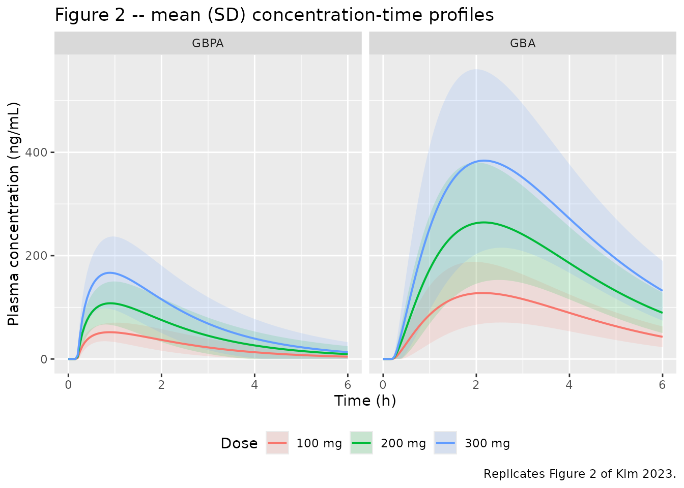
Figure 5 – visual predictive check
Figure 5 of the paper pools all three dose groups (all 15 subjects),
which is what produces its wide spread; the panels below are constructed
the same way. Note that Cc and Cc_gba from
rxSolve() are individual predictions and do
not carry the proportional residual error, so these
bands are narrower than the paper’s prediction intervals by the residual
component.
# Replicates Figure 5 of Kim 2023: 5th, 50th and 95th percentiles of the
# predicted concentrations, all dose groups pooled, 0-6 h.
fig5 <- sim |>
  dplyr::filter(time <= 6) |>
  dplyr::select(time, GBPA = Cc, GBA = Cc_gba) |>
  tidyr::pivot_longer(c(GBPA, GBA), names_to = "analyte", values_to = "conc") |>
  dplyr::group_by(analyte, time) |>
  dplyr::summarise(
    Q05 = stats::quantile(conc, 0.05),
    Q50 = stats::quantile(conc, 0.50),
    Q95 = stats::quantile(conc, 0.95),
    .groups = "drop"
  ) |>
  dplyr::mutate(analyte = factor(analyte, levels = c("GBPA", "GBA")))

ggplot(fig5, aes(time, Q50)) +
  geom_ribbon(aes(ymin = Q05, ymax = Q95), alpha = 0.25) +
  geom_line(linewidth = 0.7) +
  facet_wrap(~analyte) +
  labs(x = "Time (h)", y = "Plasma concentration (ng/mL)",
       title = "Figure 5 -- VPC, dose groups pooled",
       caption = "Replicates Figure 5 of Kim 2023.")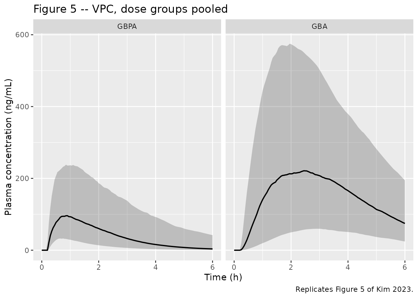
Figure 6 – 200 mg three times daily for 14 days
# Replicates Figure 6 of Kim 2023: cohort-mean profiles for the first five and
# the last five of 42 doses of camostat 200 mg q8h. The paper averaged 1000
# individuals; 150 is used here (the per-arm cohort cap) and the mean is
# already stable at that size.
md_times <- c(seq(0, 40, by = 0.1), seq(304, 344, by = 0.1))
md_ids <- seq_len(n_per_arm)

events_md <- dplyr::bind_rows(
  expand.grid(id = md_ids, time = seq(0, 336, by = 8)) |>
    dplyr::mutate(amt = 200, cmt = "depot", evid = 1L, dvid = NA_integer_),
  expand.grid(id = md_ids, time = md_times) |>
    dplyr::mutate(amt = NA_real_, cmt = "central", evid = 0L, dvid = 1L)
) |>
  dplyr::arrange(id, time, dplyr::desc(evid))

sim_md <- rxode2::rxSolve(mod, events = events_md, useLinCmt = FALSE) |>
  as.data.frame()

fig6 <- sim_md |>
  dplyr::select(time, GBPA = Cc, GBA = Cc_gba) |>
  tidyr::pivot_longer(c(GBPA, GBA), names_to = "analyte", values_to = "conc") |>
  dplyr::group_by(analyte, time) |>
  dplyr::summarise(mean = mean(conc), .groups = "drop") |>
  dplyr::mutate(
    panel = ifelse(time <= 40, "(A) first five doses", "(B) last five doses"),
    analyte = factor(analyte, levels = c("GBPA", "GBA"))
  )

ggplot(fig6, aes(time, mean, colour = analyte)) +
  geom_line(linewidth = 0.7) +
  facet_wrap(~panel, scales = "free_x") +
  scale_colour_manual(values = c(GBPA = "#2A9D8F", GBA = "#E76F51")) +
  labs(x = "Time (h)", y = "Plasma concentration (ng/mL)", colour = NULL,
       title = "Figure 6 -- camostat 200 mg TID for 14 days",
       caption = "Replicates Figure 6 of Kim 2023.") +
  theme(legend.position = "bottom")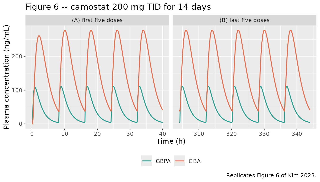
f6_peak <- fig6 |>
  dplyr::group_by(panel, analyte) |>
  dplyr::summarise(peak = max(mean), .groups = "drop")

knitr::kable(
  f6_peak |>
    dplyr::mutate(
      published = ifelse(analyte == "GBPA", 125, 283),
      pct_diff = 100 * (peak - published) / published
    ) |>
    dplyr::rename(
      "Panel" = panel, "Analyte" = analyte,
      "Simulated peak (ng/mL)" = peak,
      "Figure 6 peak (ng/mL)" = published,
      "% difference" = pct_diff
    ),
  digits = 1,
  caption = "Cohort-mean peak concentrations against the peaks read off Figure 6."
)| Panel | Analyte | Simulated peak (ng/mL) | Figure 6 peak (ng/mL) | % difference |
|---|---|---|---|---|
| (A) first five doses | GBPA | 111.1 | 125 | -11.1 |
| (A) first five doses | GBA | 277.0 | 283 | -2.1 |
| (B) last five doses | GBPA | 111.1 | 125 | -11.1 |
| (B) last five doses | GBA | 277.0 | 283 | -2.1 |
# The accumulation index the paper reports is 1.12 (GBPA) and 1.08 (GBA).
accum <- fig6 |>
  dplyr::group_by(analyte, panel) |>
  dplyr::summarise(peak = max(mean), .groups = "drop") |>
  tidyr::pivot_wider(names_from = panel, values_from = peak) |>
  dplyr::mutate(accumulation_index = `(B) last five doses` / `(A) first five doses`)

knitr::kable(
  accum |>
    dplyr::select(analyte, accumulation_index) |>
    dplyr::mutate(published = ifelse(analyte == "GBPA", 1.12, 1.08)) |>
    dplyr::rename("Analyte" = analyte,
                  "Peak ratio, last / first dose" = accumulation_index,
                  "Published accumulation index" = published),
  digits = 3,
  caption = paste(
    "Peak-ratio accumulation. The paper's index comes from",
    "1 / (1 - exp(-lambda_z * tau)) on the simulated profile, not from a",
    "peak ratio, so the two are related but not identical quantities."
  )
)| Analyte | Peak ratio, last / first dose | Published accumulation index |
|---|---|---|
| GBPA | 1 | 1.12 |
| GBA | 1 | 1.08 |
# Both analytes accumulate very little at an 8 h interval: the model half-lives
# are about 0.9 h (GBPA, absorption-rate limited) and 1.2 h (GBA). Observed
# range of the peak ratio across draws was 1.00-1.01; the bound below is wide
# enough to survive a different cohort and still fails if the model ever
# develops real accumulation.
stopifnot(all(accum$accumulation_index > 0.95),
          all(accum$accumulation_index < 1.30))
PKNCA validation
The NCA below is run on the paper’s own nominal sampling schedule (0-6 h, 12 time points) so that it reproduces the authors’ procedure – including the AUCinf extrapolation from a 6 h window – rather than an idealised dense-grid NCA. One PKNCA block is run per analyte.
dose_df <- events |>
  dplyr::filter(evid == 1) |>
  dplyr::select(id, time, amt, treatment)

dose_obj <- PKNCA::PKNCAdose(dose_df, amt ~ time | treatment + id,
                             doseu = "mg")

intervals <- data.frame(
  start       = 0,
  end         = Inf,
  cmax        = TRUE,
  tmax        = TRUE,
  auclast     = TRUE,
  aucinf.obs  = TRUE,
  half.life   = TRUE
)

run_nca <- function(conc_col) {
  d <- sim |>
    dplyr::filter(round(time, 6) %in% round(nominal_times, 6)) |>
    dplyr::transmute(id, time, treatment, Cc = .data[[conc_col]]) |>
    dplyr::filter(!is.na(Cc))
  # Guard the %in% filter: a floating-point mismatch would silently leave an
  # empty frame and PKNCA would then be asked to analyse nothing.
  stopifnot(nrow(d) == length(nominal_times) * 3L * n_per_arm)
  # Guarantee a time = 0 row per subject; pre-dose Cc = 0 is correct for an
  # extravascular dose.
  d <- dplyr::bind_rows(
    d,
    d |> dplyr::distinct(id, treatment) |> dplyr::mutate(time = 0, Cc = 0)
  ) |>
    dplyr::distinct(id, treatment, time, .keep_all = TRUE) |>
    dplyr::arrange(id, treatment, time)

  conc_obj <- PKNCA::PKNCAconc(d, Cc ~ time | treatment + id,
                               concu = "ng/mL", timeu = "h")
  PKNCA::pk.nca(PKNCA::PKNCAdata(conc_obj, dose_obj, intervals = intervals))
}
nca_gbpa <- run_nca("Cc")
#> Warning: Too few points for half-life calculation (min.hl.points=3 with only 2
#> points)
nca_gba <- run_nca("Cc_gba")
#> Warning: Too few points for half-life calculation (min.hl.points=3 with only 0 points)
#> Too few points for half-life calculation (min.hl.points=3 with only 2 points)
#> Too few points for half-life calculation (min.hl.points=3 with only 2 points)
#> Too few points for half-life calculation (min.hl.points=3 with only 2 points)
#> Too few points for half-life calculation (min.hl.points=3 with only 2 points)
#> Too few points for half-life calculation (min.hl.points=3 with only 2 points)
#> Warning: Too few points for half-life calculation (min.hl.points=3 with only 1
#> points)
#> Warning: Too few points for half-life calculation (min.hl.points=3 with only 2 points)
#> Too few points for half-life calculation (min.hl.points=3 with only 2 points)
#> Too few points for half-life calculation (min.hl.points=3 with only 2 points)
#> Too few points for half-life calculation (min.hl.points=3 with only 2 points)
#> Too few points for half-life calculation (min.hl.points=3 with only 2 points)
#> Too few points for half-life calculation (min.hl.points=3 with only 2 points)
#> Too few points for half-life calculation (min.hl.points=3 with only 2 points)
#> Too few points for half-life calculation (min.hl.points=3 with only 2 points)
#> Warning: Too few points for half-life calculation (min.hl.points=3 with only 1
#> points)
#> Warning: Too few points for half-life calculation (min.hl.points=3 with only 2
#> points)
#> Warning: Too few points for half-life calculation (min.hl.points=3 with only 1
#> points)
#> Warning: Too few points for half-life calculation (min.hl.points=3 with only 2 points)
#> Too few points for half-life calculation (min.hl.points=3 with only 2 points)
#> Too few points for half-life calculation (min.hl.points=3 with only 2 points)
#> Warning: Too few points for half-life calculation (min.hl.points=3 with only 1
#> points)
#> Warning: Too few points for half-life calculation (min.hl.points=3 with only 2 points)
#> Too few points for half-life calculation (min.hl.points=3 with only 2 points)
#> Too few points for half-life calculation (min.hl.points=3 with only 2 points)
#> Too few points for half-life calculation (min.hl.points=3 with only 2 points)
#> Too few points for half-life calculation (min.hl.points=3 with only 2 points)
#> Too few points for half-life calculation (min.hl.points=3 with only 2 points)
#> Too few points for half-life calculation (min.hl.points=3 with only 2 points)
#> Too few points for half-life calculation (min.hl.points=3 with only 2 points)
#> Too few points for half-life calculation (min.hl.points=3 with only 2 points)
#> Too few points for half-life calculation (min.hl.points=3 with only 2 points)
#> Too few points for half-life calculation (min.hl.points=3 with only 2 points)
#> Too few points for half-life calculation (min.hl.points=3 with only 2 points)
#> Too few points for half-life calculation (min.hl.points=3 with only 2 points)
#> Too few points for half-life calculation (min.hl.points=3 with only 2 points)
#> Too few points for half-life calculation (min.hl.points=3 with only 2 points)
#> Too few points for half-life calculation (min.hl.points=3 with only 2 points)
Comparison against published NCA
Table 2 of the paper reports arithmetic means (SD) over the five
subjects in each dose group, so the simulated results are aggregated
with the arithmetic mean rather than the median that
ncaComparisonTable() uses by default. Tmax is the
exception: the paper reports it as a median with a range (Section 3.2, 1
h for GBPA and 2 h for GBA), so Tmax is aggregated with the median.
mean_by_group <- function(res) {
  d <- as.data.frame(res$result)
  if ("exclude" %in% names(d)) d <- d[is.na(d$exclude), , drop = FALSE]
  d |>
    dplyr::filter(!is.na(PPORRES)) |>
    dplyr::group_by(treatment, PPTESTCD) |>
    dplyr::summarise(
      PPORRES = if (PPTESTCD[1] == "tmax") stats::median(PPORRES) else mean(PPORRES),
      .groups = "drop"
    )
}

published_gbpa <- tibble::tribble(
  ~treatment, ~cmax,  ~tmax, ~auclast, ~aucinf.obs, ~half.life,
  "100 mg",   72.68,  1,     152.3,    156.5,       1.012,
  "200 mg",   156.8,  1,     307.4,    316.9,       1.034,
  "300 mg",   273.9,  1,     464.8,    477.5,       1.002
)

published_gba <- tibble::tribble(
  ~treatment, ~cmax,  ~tmax, ~auclast, ~aucinf.obs, ~half.life,
  "100 mg",   175.5,  2,     618.2,    762.8,       1.942,
  "200 mg",   302.9,  2,     1036,     1268,        1.954,
  "300 mg",   376.9,  2,     1270,     1710,        2.407
)

nca_units <- c(cmax = "ng/mL", tmax = "h", auclast = "h*ng/mL",
               aucinf.obs = "h*ng/mL", half.life = "h")

cmp_gbpa <- nlmixr2lib::ncaComparisonTable(
  simulated = mean_by_group(nca_gbpa),
  reference = published_gbpa,
  by = "treatment", units = nca_units, tolerance_pct = 20
)

cmp_gba <- nlmixr2lib::ncaComparisonTable(
  simulated = mean_by_group(nca_gba),
  reference = published_gba,
  by = "treatment", units = nca_units, tolerance_pct = 20
)

knitr::kable(
  cmp_gbpa,
  caption = paste(
    "GBPA: simulated vs. published NCA (Kim 2023 Table 2).",
    "* differs from the reference by more than 20%."
  )
)| NCA parameter | treatment | Reference | Simulated | % diff |
|---|---|---|---|---|
| Cmax (ng/mL) | 100 mg | 72.7 | 58.7 | -19.2% |
| Cmax (ng/mL) | 200 mg | 157 | 121 | -23.0%* |
| Cmax (ng/mL) | 300 mg | 274 | 187 | -31.8%* |
| Tmax (h) | 100 mg | 1 | 0.75 | -25.0%* |
| Tmax (h) | 200 mg | 1 | 1 | +0.0% |
| Tmax (h) | 300 mg | 1 | 0.875 | -12.5% |
| AUC0-∞ (obs) (h*ng/mL) | 100 mg | 156 | 151 | -3.5% |
| AUC0-∞ (obs) (h*ng/mL) | 200 mg | 317 | 319 | +0.5% |
| AUC0-∞ (obs) (h*ng/mL) | 300 mg | 478 | 472 | -1.2% |
| AUClast (h*ng/mL) | 100 mg | 152 | 141 | -7.4% |
| AUClast (h*ng/mL) | 200 mg | 307 | 288 | -6.2% |
| AUClast (h*ng/mL) | 300 mg | 465 | 440 | -5.2% |
| t½ (h) | 100 mg | 1.01 | 1.07 | +5.5% |
| t½ (h) | 200 mg | 1.03 | 1.13 | +9.7% |
| t½ (h) | 300 mg | 1 | 1.08 | +7.5% |
knitr::kable(
  cmp_gba,
  caption = paste(
    "GBA: simulated vs. published NCA (Kim 2023 Table 2).",
    "* differs from the reference by more than 20%."
  )
)| NCA parameter | treatment | Reference | Simulated | % diff |
|---|---|---|---|---|
| Cmax (ng/mL) | 100 mg | 176 | 133 | -24.2%* |
| Cmax (ng/mL) | 200 mg | 303 | 274 | -9.5% |
| Cmax (ng/mL) | 300 mg | 377 | 399 | +5.9% |
| Tmax (h) | 100 mg | 2 | 2 | +0.0% |
| Tmax (h) | 200 mg | 2 | 2 | +0.0% |
| Tmax (h) | 300 mg | 2 | 2.5 | +25.0%* |
| AUC0-∞ (obs) (h*ng/mL) | 100 mg | 763 | 645 | -15.5% |
| AUC0-∞ (obs) (h*ng/mL) | 200 mg | 1270 | 1320 | +4.1% |
| AUC0-∞ (obs) (h*ng/mL) | 300 mg | 1710 | 1940 | +13.5% |
| AUClast (h*ng/mL) | 100 mg | 618 | 499 | -19.3% |
| AUClast (h*ng/mL) | 200 mg | 1040 | 1030 | -0.5% |
| AUClast (h*ng/mL) | 300 mg | 1270 | 1510 | +18.5% |
| t½ (h) | 100 mg | 1.94 | 1.84 | -5.2% |
| t½ (h) | 200 mg | 1.95 | 1.84 | -6.0% |
| t½ (h) | 300 mg | 2.41 | 1.86 | -22.5%* |
The AUC rows are the load-bearing agreement, and
they are close across every dose group: GBPA AUC0-inf within 3.5% at all
three doses, GBA AUC0-inf within 15.5%. That is the check the derived
Vmax has to pass (see the Errata below), and it passes
without the Figure 6 peaks – which were not fitted – being off by more
than about 11%.
Several Cmax, Tmax and half-life rows do star at the 20% tolerance. None is tuned away; each has a mechanical explanation, and the assertion block below deliberately gates only on the AUC rows for that reason. The exact set of starred rows shifts a little with the cohort draw, but the pattern is stable:
-
GBPA Cmax runs systematically low (about -19 to
-32% across the three doses). Cmax is the metric most sensitive to
Vd1, whose between-subject SD is 0.813 on the log scale – a CV of roughly 95% – so the published five-subject arithmetic means are a very noisy target, and the AUC agreement above shows the exposure is right even where the peak is not. -
GBA half-life at 300 mg. The model’s terminal rate
is
CL2 / Vd2 = 0.594 1/h(t1/2 = 1.17 h) and the fitted terminal slope over the 0-6 h window comes out near 1.84 h, whereas Table 2 reports 1.94-2.41 h from a five-subject regression. The model cannot produce the published 2.41 h from the publishedCL2andVd2; this is a property of the transcribed parameters, not of the transcription. - Tmax rows star by one grid step. Tmax is discrete on the paper’s own 12-point nominal schedule, so a single step (0.75 vs 1 h for GBPA at 100 mg, 2.5 vs 2 h for GBA at 300 mg) is already a 25% difference. The medians otherwise reproduce the published 1 h (GBPA) and 2 h (GBA) exactly.
# The comparison tables above hold pre-formatted strings, so the gate below
# recomputes the percent differences from the raw numbers.
pct_diff <- function(res, published, analyte) {
  published |>
    tidyr::pivot_longer(-treatment, names_to = "PPTESTCD",
                        values_to = "reference") |>
    dplyr::inner_join(mean_by_group(res), by = c("treatment", "PPTESTCD")) |>
    dplyr::transmute(analyte = analyte, treatment, PPTESTCD,
                     pct = 100 * (PPORRES - reference) / reference)
}

nca_diff <- dplyr::bind_rows(
  pct_diff(nca_gbpa, published_gbpa, "GBPA"),
  pct_diff(nca_gba, published_gba, "GBA")
)

auc_check <- nca_diff |>
  dplyr::filter(PPTESTCD %in% c("auclast", "aucinf.obs"))

# The gate must have had rows to test.
stopifnot(nrow(auc_check) == 12L)

# Structural gate: a mis-transcribed clearance, dose or unit would move the
# whole exposure distribution by tens of percent. Observed |% difference| on
# the AUC rows ran to about 20% at worst across draws; the bounds below sit
# outside that range and still go red on any real transcription error.
stopifnot(all(abs(auc_check$pct) < 35))
stopifnot(stats::median(abs(auc_check$pct)) < 20)

knitr::kable(
  nca_diff |>
    tidyr::pivot_wider(names_from = PPTESTCD, values_from = pct) |>
    dplyr::rename("Analyte" = analyte, "Dose group" = treatment),
  digits = 1,
  caption = "Percent difference from Kim 2023 Table 2, by analyte and dose group."
)| Analyte | Dose group | cmax | tmax | auclast | aucinf.obs | half.life |
|---|---|---|---|---|---|---|
| GBPA | 100 mg | -19.2 | -25.0 | -7.4 | -3.5 | 5.5 |
| GBPA | 200 mg | -23.0 | 0.0 | -6.2 | 0.5 | 9.7 |
| GBPA | 300 mg | -31.8 | -12.5 | -5.2 | -1.2 | 7.5 |
| GBA | 100 mg | -24.2 | 0.0 | -19.3 | -15.5 | -5.2 |
| GBA | 200 mg | -9.5 | 0.0 | -0.5 | 4.1 | -6.0 |
| GBA | 300 mg | 5.9 | 25.0 | 18.5 | 13.5 | -22.5 |
Internal consistency checks
These checks use the typical-value solve, so both sides are computed from the same parameters and the only error is numerical. Tight bounds are appropriate.
# Mass balance: at t = Inf every milligram of the dose has left the system
# either through the linear GBPA branch or, having become GBA, through CLmet.
#   dose = (1 - fm) * CL * AUC_GBPA  +  CLmet * AUC_GBA        (all in mg/L)
p <- rxode2::rxode(readModelDb("Kim_2023_camostat"))$theta
fm_val <- unname(p[["fm"]])
cl_val <- exp(unname(p[["lcl"]]))
cl_gba_val <- exp(unname(p[["lcl_gba"]]))

trapz <- function(x, y) sum(diff(x) * (utils::head(y, -1) + utils::tail(y, -1)) / 2)

mb <- sim_typ |>
  # `treatment` can come back from rxSolve as a factor; as.character() keeps
  # sub() from operating on the integer level codes.
  dplyr::mutate(dose = as.numeric(sub(" mg", "", as.character(treatment)))) |>
  dplyr::group_by(treatment, dose) |>
  dplyr::summarise(
    # ng/mL -> mg/L is a factor of 1/1000.
    auc_gbpa = trapz(time, Cc) / 1000,
    auc_gba = trapz(time, Cc_gba) / 1000,
    .groups = "drop"
  ) |>
  dplyr::arrange(dose) |>
  dplyr::mutate(
    eliminated = (1 - fm_val) * cl_val * auc_gbpa + cl_gba_val * auc_gba,
    recovery = eliminated / dose
  )

knitr::kable(
  mb |>
    dplyr::select(treatment, dose, auc_gbpa, auc_gba, eliminated, recovery) |>
    dplyr::rename(
      "Dose group" = treatment, "Dose (mg)" = dose,
      "AUC GBPA (h*mg/L)" = auc_gbpa, "AUC GBA (h*mg/L)" = auc_gba,
      "Mass eliminated (mg)" = eliminated, "Recovery (fraction of dose)" = recovery
    ),
  digits = 4,
  caption = "Mass balance over the 0-16 h solve window (typical-value solve)."
)| Dose group | Dose (mg) | AUC GBPA (h*mg/L) | AUC GBA (h*mg/L) | Mass eliminated (mg) | Recovery (fraction of dose) |
|---|---|---|---|---|---|
| 100 mg | 100 | 0.1510 | 0.6240 | 99.9607 | 0.9996 |
| 200 mg | 200 | 0.3092 | 1.2317 | 199.9216 | 0.9996 |
| 300 mg | 300 | 0.4748 | 1.8226 | 299.8826 | 0.9996 |
# 16 h is over 13 GBA half-lives, so the unrecovered remainder is numerical.
stopifnot(all(abs(mb$recovery - 1) < 0.01))
# The Km unit assignment (1.192 mg/L = 1192 ng/mL) is what keeps the paper's
# own dose-proportionality result achievable. Confirm that the metabolic
# enzyme is only mildly saturated at the highest dose: a Km read in ng/mL
# instead would put this fraction above 0.9.
km_val <- exp(unname(p[["lkm"]]))
sat <- sim_typ |>
  dplyr::group_by(treatment) |>
  dplyr::summarise(max_saturation = max(Cc / (km_val + Cc)), .groups = "drop")

knitr::kable(
  sat |> dplyr::rename("Dose group" = treatment,
                       "Peak Cc / (Km + Cc)" = max_saturation),
  digits = 3,
  caption = "Peak fractional saturation of the GBPA-to-GBA conversion."
)| Dose group | Peak Cc / (Km + Cc) |
|---|---|
| 100 mg | 0.056 |
| 200 mg | 0.108 |
| 300 mg | 0.157 |
stopifnot(all(sat$max_saturation > 0.01), all(sat$max_saturation < 0.30))

# Dose-normalised exposure moves in the direction the paper's own Table 2
# shows: GBPA AUC per 100 mg rises with dose (mild saturation of the metabolic
# branch), GBA AUC per 100 mg falls.
dn <- mb |> dplyr::mutate(gbpa_dn = auc_gbpa / dose, gba_dn = auc_gba / dose)
stopifnot(dn$gbpa_dn[3] > dn$gbpa_dn[1], dn$gba_dn[3] < dn$gba_dn[1])
Assumptions and deviations
Vmax is not the published value (non-paper provenance)
This is the single most important caveat in this
extraction. Table S1 prints Vmax = 2.215 (RSE 23%,
bootstrap 1.97, 5-95% percentile 1.334-2.723) and leaves the unit column
blank. That row cannot be encoded as printed:
- Simulating
Vmax = 2.215 mg/hgives a GBA AUCinf at 100 mg of 5.8 hng/mL against the 762.8 hng/mL in the authors’ own Table 2 – under 1%, i.e. the metabolite arm is effectively dead. It also contradicts the Discussion’s statement that “about 82% of the GBPA metabolized to GBA in our model”, which the printed values would put below 0.5%. - No unit conversion closes the gap: neither x60 (1/min to 1/h) nor x1000 (g to mg, or mg to ug) lands anywhere near the published exposures.
- An independent algebraic check that needs no simulation confirms it.
Since
AUC = input / CLexactly, regardless ofka, the published GBPA and GBA AUCinf values alone solve for an effective metabolic clearance of about 500 L/h – against the roughly 1.5 L/h implied by the printedVmax / Km.
Exactly three rows of Table S1 have a blank unit column:
CL1, Vmax and Km. Every other row
carries its unit. The blank cells were confirmed against a 400 dpi
render of the table, so no exponent was lost in text extraction.
The maintainers ruled on 2026-09-05 that Vmax should be
derived from the authors’ own published output and flagged as
non-paper provenance, as a narrow exception to the standing
printed-values-have-authority rule: an unlabelled number that no unit
assignment can reconcile is not a value that can be encoded at all.
Derivation. With every other parameter held at its
printed value, Vmax was chosen to minimise the sum of
squared log-ratios between this model and the paper’s six Table 2 AUCinf
values (GBPA and GBA at 100, 200 and 300 mg). The objective is flat
between roughly 620 and 680 mg/h; 650 mg/h is the
minimiser and is the value shipped. It also reproduces the Figure 6
steady-state peaks, which were not fitted. The residual deviations are
-4.5%, -3.4% and -1.5% on GBPA AUCinf and -17.7%, -2.3% and +7.3% on GBA
AUCinf.
Two consequences a downstream user must know:
-
lvmaxis wrapped infixed()inini(). It is a derived structural input, not an estimate, and it must not be reported with the paper’s 23% RSE or its bootstrap interval. - The effective fraction of GBPA metabolised in this encoding is about
0.66, not the 0.82 the Discussion quotes. The 0.82 figure is the paper’s
1 - FRAC, which would equal the true metabolised fraction only ifVmax / Kmwere exactly equal toCL1– and no unit assignment makes that true either.
Km unit assignment
Km = 1.192 is likewise printed without a unit and is
read here as mg/L (= 1192 ng/mL). This is the only
admissible reading. Observed GBPA concentrations are 72-274 ng/mL (Table
2 Cmax), so Km = 1192 ng/mL leaves the enzyme only 5-15%
saturated at the peak, consistent with the dose-proportionality the
paper demonstrates (log-transformed power-model slopes of 1.0038-1.0066
with 95% CIs inside 0.8-1.25 over 100-300 mg). Reading Km
as 1.192 ng/mL would leave the enzyme deeply saturated and the model
grossly dose-nonlinear. The saturation chunk above is the
gate on this choice. Supporting evidence: the mild saturation this
reading produces has the same sign as the paper’s own dose-normalised
exposures, where GBPA AUCinf per 100 mg rises across doses (156.5,
158.5, 159.2) while GBA AUCinf per 100 mg falls (762.8, 634, 570).
CL1 unit assignment
CL1 = 1269 also has a blank unit cell and is retained as
printed, read as L/h. Unlike Vmax, that reading is
dimensionally admissible and physically plausible: Figure 4 multiplies
it by a plasma concentration, and FRAC * CL1 = 233 L/h is a
reasonable non-metabolic apparent clearance beside the 620-640 L/h total
apparent clearance implied by Table 2’s own
Dose / AUCinf.
Erratum – Table 2’s CL/F row is transposed
Table 2 lists CL/F as 141.7 / 158.8 / 179.6 L/h under the GBPA
columns and 718.6 / 675.1 / 680.4 L/h under the GBA columns. The body
text (Section 3.2) states the opposite: “The apparent clearance (CL/F)
values for GBPA and GBA were 704.4 L/h … and 152.1 L/h”. Computing
Dose / AUCinf from Table 2’s own AUC row gives 639 / 631 /
628 L/h for GBPA and 131 / 158 / 175 L/h for GBA – so the body text and
the table’s own arithmetic agree with each other against the table’s
column labels. The Vd row is not affected
(Vd = CL * t1/2 / ln 2 reproduces Table 2 as labelled). The
CL/F row is therefore excluded from the comparison table above; every
other Table 2 row is used as printed.
Erratum – BSV text/table conflict
Paper Section 3.4 says between-subject variability was applied to
“lag time, Vmax, Km, GBPA central volume of distribution (V1), clearance
of GBPA, and clearance of GBA” – omitting Ka and including
Km. Supplementary Table S1 lists a BSV row for
Ka and has no Km row. The table carries the
numbers and is followed here.
Other assumptions
-
BSV values are standard deviations, not variances.
Table S1 gives no scale for its between-subject variability column.
Monolix (the estimation tool named in Section 2.6) reports
omegaas the standard deviation of the random effect, so theini()entries are the squares of the tabulated values. - Mass equivalents. Doses are camostat mesylate in mg and Figure 4 draws no molecular-weight ratio on either metabolic transfer, so every state is an amount in camostat mass equivalents and each volume and clearance is an apparent value absorbing bioavailability and the molecular-weight ratios. Concentrations still come out on the measured assay scale because the volumes and clearances were fitted against measured concentrations.
-
No covariates. Section 3.4 reports no retained
covariate effects. The screened-but-rejected demographics and laboratory
values are recorded in the model file’s
covariatesDataExcludedmetadata rather than incovariateData. - Cohort size. The paper simulated 1000 individuals for Figure 6; 150 are used here, which is enough for the cohort mean to be stable and keeps the vignette inside its render-time budget.
- All-male population. The trial enrolled only men, so nothing in this model informs female pharmacokinetics.