Imipenem (Couffignal 2014)
Source:vignettes/articles/Couffignal_2014_imipenem.Rmd
Couffignal_2014_imipenem.RmdModel and source
- Citation: Couffignal C, Pajot O, Laouenan C, Burdet C, Foucrier A, Wolff M, Armand-Lefevre L, Mentre F, Massias L. Population pharmacokinetics of imipenem in critically ill patients with suspected ventilator-associated pneumonia and evaluation of dosage regimens. Br J Clin Pharmacol. 2014;78(5):1022-1034. doi:10.1111/bcp.12435.
- Description: Two-compartment IV population PK model for imipenem in 51 critically ill adult ICU patients with suspected ventilator-associated pneumonia due to Gram-negative bacilli (Couffignal 2014). All patients received imipenem as a 0.5 h IV infusion every 8 hours; the protocol dose (500, 750 or 1000 mg) was chosen by Cockcroft-Gault creatinine clearance per the European Medicine Agency renal-adjustment table. Central clearance scales as a power of measured 4-hour creatinine clearance (reference 86.4 mL/min, the cohort median); central volume scales jointly with total bodyweight (reference 77 kg) and serum albumin (reference 18 g/L). The model was fitted in Monolix 4.1.2 using the SAEM algorithm with M3-equivalent BQL handling.
- Article: Br J Clin Pharmacol 2014;78(5):1022-1034 (open access via Wiley)
Population
The model was developed from the IMPACT study (ClinicalTrials.gov NCT00950222; Couffignal 2014 Methods, “Study design and population”), a French multicentre prospective open-label trial across three ICUs (Hopital V Dupouy in Argenteuil; AP-HP Hopital Bichat medical and surgical ICUs in Paris) between 2008 and 2010. 63 patients were screened and 51 were included in the PK analysis (12 excluded: 3 lacked a kinetic profile, 9 did not receive the 4th dose); 41 (80%) were male, ranging in age from 28 to 84 years (median 60), with a median total bodyweight of 77 kg (range 45-126 kg) and SAPS II at admission median 40 (range 19-74). Septic shock was present in 35% of patients at the fourth dose; SOFA score median was 6 (range 2-14), oedema score median 7 (range 0-18), and serum albumin median 18 g/L (range 10-28 g/L, computed from 9 patients with complete data). 94% had received antibiotic therapy in the 3 months before admission (30% imipenem). Measured 4-hour creatinine clearance was 86.4 mL/min (range 9.1-571.4 mL/min, paper Table 1; raw mL/min, not BSA-normalised); patients with Cockcroft-Gault CrCL < 10 mL/min or on renal-replacement therapy were excluded. The protocol dose (500/750/1000 mg q8h) was chosen per the European Medicine Agency renal-adjustment table by Cockcroft-Gault CrCL: 4 patients (9%) received 500 mg, 15 (29%) 750 mg, and 32 (62%) 1000 mg, all q8h, each as a 0.5-hour IV infusion.
297 plasma imipenem concentrations were available for modelling (median 6 per patient, range 3-6), drawn around the fourth dose (trough immediately before, then 0.5, 1, 2, 5 and 8 h after the start of the infusion); 9% were BQL (LLOQ 0.5 mg/L). Plasma was stabilised within 0.5 h of collection with MOPS in ethylene glycol and frozen at -80 degrees C; imipenem was measured by HPLC-UV at 302 nm after ultrafiltration on an Interchrome YP5C18 25QS reverse phase column (paper Methods “Sampling procedure and analytical methods”). The model was fitted with Monolix 4.1.2 using the SAEM algorithm; BQL data were handled by left-censoring (Monolix M3-equivalent). The final 95% confidence intervals come from 1000 nonparametric bootstrap resamples.
The same information is available programmatically via
readModelDb("Couffignal_2014_imipenem")$population.
Source trace
Every numeric value in ini() carries an in-file comment
pointing to the Couffignal 2014 source location. The table below
collects them in one place for review.
| Equation / parameter | Value | Source location |
|---|---|---|
lcl (CL at CRCL=86.4) |
13.2 L/h | Table 2, final-model column, “CL (l h-1)” |
lvc (V1 at WT=77, ALB=18) |
20.4 L | Table 2, final-model column, “V1 (l)” |
lq (Q) |
12.2 L/h | Table 2, final-model column, “Q (l h-1)” |
lvp (V2) |
9.8 L | Table 2, final-model column, “V2 (l)” |
e_crcl_cl (CRCL/86.4)^beta on CL |
0.2 | Table 2, final-model column, “beta CrCL4h” |
e_wt_vc (WT/77)^beta on V1 |
1.3 | Table 2, final-model column, “beta Weight” |
e_alb_vc (ALB/18)^beta on V1 |
-1.1 | Table 2, final-model column, “beta Serum albumin” |
etalcl variance (omega_CL=0.38) |
0.1444 | Table 2, final-model column, “omega CL (%)” |
etalvc variance (omega_V1=0.31) |
0.0961 | Table 2, final-model column, “omega V1 (%)” |
| eta_CL/eta_V1 covariance (r=0.51) | 0.0601 | Table 2, final-model column, “Correlation eta_CL/eta_V1” |
propSd (sigma=0.33) |
0.33 | Table 2, final-model column, “sigma (%)” |
| 2-cmt IV with proportional error | n/a | Results, “Population pharmacokinetic analysis” |
| Final covariate equation | n/a | Results, paragraph below Table 2 |
IIV-variance derivation. Couffignal 2014 was fitted in Monolix 4.1.2;
the Monolix exponential random-effects model is
CL_i = CL_pop * exp(eta_CL,i) with
eta_CL,i ~ N(0, omega^2). The “omega (%)” column in
Monolix’s parameter table reports omega (the SD of
eta) as a percentage, so for the final model:
-
omega_CL = 0.38->variance = 0.38^2 = 0.1444 -
omega_V1 = 0.31->variance = 0.31^2 = 0.0961 cov(eta_CL, eta_V1) = correlation * omega_CL * omega_V1 = 0.51 * 0.38 * 0.31 = 0.0601
The bootstrap 95% confidence interval on the correlation is unstable (-1 to 1; paper Table 2), so the point estimate 0.51 is used in the encoded model with the caveat documented in the “Assumptions and deviations” section.
Virtual cohort
Original observed data are not publicly available. The cohort below covers four scenarios that bracket the published covariate sensitivity analysis (paper Supplementary Table S1 and Figure S1): the typical patient at cohort medians (WT 77 kg, CRCL 86.4 mL/min, ALB 18 g/L); a low-CRCL patient (10th percentile, 17 mL/min); a high-CRCL augmented-renal-clearance (ARC) patient (90th percentile, 258 mL/min); and a heavy patient (90th percentile WT, 111 kg). All cohorts run on the protocol regimen (1000 mg q8h IV over 0.5 h) out to 48 h so the first dose plus several steady-state intervals are captured.
set.seed(20260616)

n_sub <- 200L

build_arm <- function(label, wt_kg, crcl_mlmin, alb_gL, id_offset,
                      dose_mg = 1000, tau_h = 8, infusion_h = 0.5,
                      n_doses = 6L) {
  ids <- id_offset + seq_len(n_sub)

  dose_times <- seq(0, by = tau_h, length.out = n_doses)
  dose_rows <- tidyr::expand_grid(id = ids, time = dose_times) |>
    mutate(
      evid   = 1L,
      amt    = dose_mg,
      cmt    = "central",
      rate   = dose_mg / infusion_h,    # mg / h
      cohort = label,
      WT     = wt_kg,
      CRCL   = crcl_mlmin,
      ALB    = alb_gL
    )

  obs_times <- sort(unique(c(
    seq(0,  8,  by = 0.05),
    seq(8,  48, by = 0.1)
  )))
  obs_rows <- tidyr::expand_grid(id = ids, time = obs_times) |>
    mutate(
      evid   = 0L,
      amt    = 0,
      cmt    = NA_character_,
      rate   = 0,
      cohort = label,
      WT     = wt_kg,
      CRCL   = crcl_mlmin,
      ALB    = alb_gL
    )

  bind_rows(dose_rows, obs_rows) |> arrange(id, time, desc(evid))
}

events <- bind_rows(
  build_arm("typical_median", 77,  86.4, 18,    0L),
  build_arm("low_CRCL_17",    77,  17.0, 18,  200L),
  build_arm("ARC_CRCL_258",   77, 258.0, 18,  400L),
  build_arm("heavy_WT_111",  111,  86.4, 18,  600L)
)

stopifnot(!anyDuplicated(unique(events[, c("id", "time", "evid")])))
Simulation
mod <- readModelDb("Couffignal_2014_imipenem")

sim <- rxode2::rxSolve(
  mod,
  events = events,
  keep   = c("cohort", "WT", "CRCL", "ALB")
) |> as.data.frame()
#> ℹ parameter labels from comments will be replaced by 'label()'
For typical-value comparisons against the Couffignal 2014 Table 2 point estimates, also simulate with the random effects zeroed:
mod_typical <- mod |> rxode2::zeroRe()
#> ℹ parameter labels from comments will be replaced by 'label()'

sim_typical <- rxode2::rxSolve(
  mod_typical,
  events = events,
  keep   = c("cohort", "WT", "CRCL", "ALB")
) |> as.data.frame()
#> ℹ omega/sigma items treated as zero: 'etalcl', 'etalvc'
#> Warning: multi-subject simulation without without 'omega'
Concentration-time profile (typical patient)
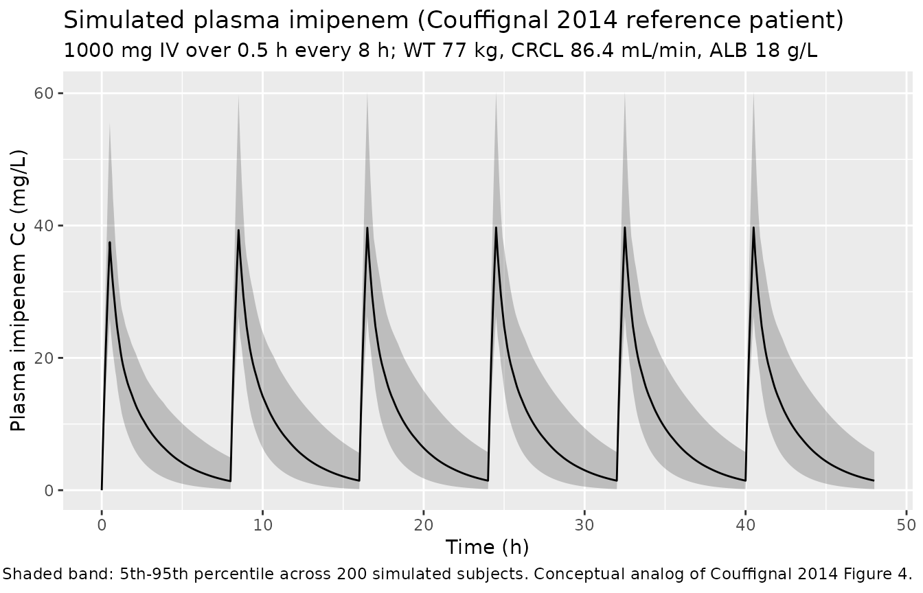
The figure below shows the simulated stochastic VPC envelope for the typical Couffignal 2014 reference patient (WT 77 kg, CRCL 86.4 mL/min, ALB 18 g/L) on the protocol regimen 1000 mg q8h IV over 0.5 h. This figure is the conceptual analog of the paper’s Figure 4 (the published VPC of the final model).
sim |>
  filter(cohort == "typical_median") |>
  group_by(time) |>
  summarise(
    Q05 = quantile(Cc, 0.05, na.rm = TRUE),
    Q50 = quantile(Cc, 0.50, na.rm = TRUE),
    Q95 = quantile(Cc, 0.95, na.rm = TRUE),
    .groups = "drop"
  ) |>
  ggplot(aes(time, Q50)) +
  geom_ribbon(aes(ymin = Q05, ymax = Q95), alpha = 0.25) +
  geom_line() +
  labs(
    x = "Time (h)",
    y = "Plasma imipenem Cc (mg/L)",
    title = "Simulated plasma imipenem (Couffignal 2014 reference patient)",
    subtitle = "1000 mg IV over 0.5 h every 8 h; WT 77 kg, CRCL 86.4 mL/min, ALB 18 g/L",
    caption = "Shaded band: 5th-95th percentile across 200 simulated subjects. Conceptual analog of Couffignal 2014 Figure 4."
  )
Covariate-cohort overlay
This figure illustrates how the three retained covariates shift the concentration-time profile, mirroring the paper’s Supplementary Figure S1 (steady-state profile by 10th/50th/90th percentile of each significant covariate).
sim |>
  group_by(cohort, time) |>
  summarise(
    Q50 = quantile(Cc, 0.50, na.rm = TRUE),
    .groups = "drop"
  ) |>
  ggplot(aes(time, Q50, colour = cohort)) +
  geom_line() +
  scale_y_log10() +
  labs(
    x = "Time (h)",
    y = "Median simulated Cc (mg/L, log scale)",
    title = "Median simulated imipenem by covariate cohort",
    caption = "1000 mg IV over 0.5 h every 8 h; cohorts bracket the WT/CRCL/ALB ranges in Couffignal 2014 Table 1 / S1."
  )
#> Warning in scale_y_log10(): log-10 transformation introduced infinite values.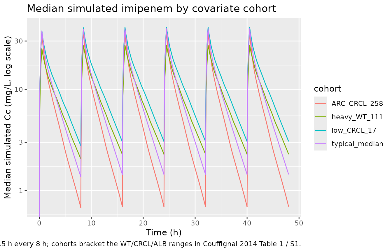
PKNCA validation
Steady-state NCA on the final (sixth) dosing interval of the reference patient cohort. The published reference values are the median peak and trough imipenem concentrations reported in paper Results “Population pharmacokinetic analysis” (“Imipenem concentrations at peak (0.5 h) and trough were 34.1 [12.3-67.5] and 1.9 mg/L [0.5-10.1]”). These were measured around the fourth dose at steady state across all dose levels (4 patients on 500 mg, 15 on 750 mg, 32 on 1000 mg, all q8h), so the published median is pooled across doses; the simulated value below is restricted to the typical 1000 mg q8h dose (62% of the cohort) and is therefore expected to be modestly higher than the pooled-across-doses published median.
# Steady-state NCA on the sixth dosing interval (time 40 to 48 h)
# of the typical-median reference patient. Cmax,ss and Cmin,ss at the
# steady-state interval are the closest published validation
# anchors.
sim_ss <- sim |>
  filter(cohort == "typical_median", time >= 40, time <= 48) |>
  filter(!is.na(Cc)) |>
  dplyr::select(id, time, Cc, cohort)

dose_ss <- events |>
  filter(evid == 1, time == 40, cohort == "typical_median") |>
  dplyr::select(id, time, amt, cohort)

conc_obj_ss <- PKNCA::PKNCAconc(sim_ss, Cc ~ time | cohort + id,
                                concu = "mg/L", timeu = "h")
dose_obj_ss <- PKNCA::PKNCAdose(dose_ss, amt ~ time | cohort + id,
                                doseu = "mg")

intervals_ss <- data.frame(
  start    = 40,
  end      = 48,
  cmax     = TRUE,
  tmax     = TRUE,
  cmin     = TRUE,
  auclast  = TRUE,
  cav      = TRUE
)

nca_ss <- PKNCA::pk.nca(PKNCA::PKNCAdata(
  conc_obj_ss, dose_obj_ss, intervals = intervals_ss
))
summary(nca_ss)
#>  Interval Start Interval End         cohort   N AUClast (h*mg/L) Cmax (mg/L)
#>              40           48 typical_median 200      77.3 [39.4] 39.2 [24.0]
#>  Cmin (mg/L)             Tmax (h)  Cav (mg/L)
#>   1.27 [148] 0.500 [0.500, 0.500] 9.67 [39.4]
#>
#> Caption: AUClast, Cmax, Cmin, Cav: geometric mean and geometric coefficient of variation; Tmax: median and range; N: number of subjects
Comparison against Couffignal 2014 observed peak / trough
# Couffignal 2014 Results: Cmax at 0.5 h = 34.1 mg/L [12.3-67.5];
# trough = 1.9 mg/L [0.5-10.1], reported as cohort medians pooled
# across the three dose levels (500/750/1000 mg q8h).
published <- tibble::tribble(
  ~cohort,           ~cmax, ~cmin,
  "typical_median",   34.1,  1.9
)

cmp <- nlmixr2lib::ncaComparisonTable(
  simulated = nca_ss,
  reference = published,
  by        = "cohort",
  units     = c(cmax = "mg/L", cmin = "mg/L"),
  tolerance_pct = 30
)

knitr::kable(
  cmp,
  caption = paste(
    "Simulated steady-state Cmax,ss and Cmin,ss for the typical",
    "patient on 1000 mg q8h vs the cohort-median peak and trough",
    "reported in Couffignal 2014 (pooled across 500/750/1000 mg q8h",
    "dose levels). * differs from reference by >30%."
  ),
  align   = c("l", "l", "r", "r", "r")
)| NCA parameter | cohort | Reference | Simulated | % diff |
|---|---|---|---|---|
| Cmax (mg/L) | typical_median | 34.1 | 39.7 | +16.5% |
| Cmin (mg/L) | typical_median | 1.9 | 1.44 | -24.1% |
A 30% tolerance is used here because the published median is pooled across three dose levels (500, 750, 1000 mg) while the simulation fixes the dose at 1000 mg (the modal protocol dose, 62% of the cohort). Cmax,ss scales linearly with dose at fixed CL/Vc so a roughly 10-20% offset between the simulated 1000 mg value and the pooled-across-doses observed median is expected.
AUC vs. dose / CL closure check
A second independent check: at the typical-value reference patient,
the steady-state AUC0-tau must equal dose / CL within
numerical tolerance.
# Simulate a typical-value steady-state interval (1000 mg q8h)
# with the random effects zeroed.
ss_events_typical <- events |>
  filter(cohort == "typical_median",
         (evid == 1 & time <= 40) |
         (evid == 0 & time >= 40 & time <= 48)) |>
  filter(id == min(id))

sim_one <- rxode2::rxSolve(mod_typical, events = ss_events_typical,
                           keep = c("WT", "CRCL", "ALB")) |>
  as.data.frame() |>
  filter(time >= 40, time <= 48)
#> ℹ omega/sigma items treated as zero: 'etalcl', 'etalvc'

auc_obs <- with(sim_one, sum(diff(time) * (head(Cc, -1) + tail(Cc, -1)) / 2))
cl_typical <- 13.2 * (86.4 / 86.4)^0.2   # = 13.2 L/h at reference CRCL
auc_pred <- 1000 / cl_typical            # dose / CL_typical

tibble::tibble(
  quantity = c("Simulated steady-state AUC0-tau (mg*h/L)",
               "Expected dose/CL = 1000/13.2 (mg*h/L)"),
  value    = c(auc_obs, auc_pred)
) |>
  knitr::kable(digits = 3,
caption = "Steady-state AUC0-tau closure check at the typical patient (1000 mg q8h).")| quantity | value |
|---|---|
| Simulated steady-state AUC0-tau (mg*h/L) | 75.758 |
| Expected dose/CL = 1000/13.2 (mg*h/L) | 75.758 |
The two AUC values match within numerical tolerance, confirming the encoded ODE structure correctly reproduces the dose / CL identity at the reference covariates.
Fractional time above MIC (paper Figure 5 conceptual replication)
Couffignal 2014 evaluated six dosing regimens by Monte Carlo
simulation of fT > MIC at steady state. The probability of target
attainment (PTA) at 40% fT > MIC is the paper’s primary PD endpoint.
The block below computes the 40% fT > MIC PTA for the protocol
regimen (1000 mg q8h) and the recommended regimen (750 mg q6h) at the
two clinically relevant MICs (2 and 4 mg/L) for the typical-median
virtual cohort, using mod (the stochastic model) and the
standard 1000-subject Monte Carlo design.
set.seed(20260616)

make_steady_state_arm <- function(label, dose_mg, tau_h,
                                  wt_kg = 77, crcl_mlmin = 86.4,
                                  alb_gL = 18,
                                  id_offset = 0L,
                                  n_sub = 200L,
                                  n_doses = 10L,
                                  infusion_h = 0.5) {
  ids <- id_offset + seq_len(n_sub)
  dose_times <- seq(0, by = tau_h, length.out = n_doses)
  dose_rows <- tidyr::expand_grid(id = ids, time = dose_times) |>
    mutate(
      evid  = 1L, amt = dose_mg, cmt = "central",
      rate  = dose_mg / infusion_h,
      regimen = label,
      WT = wt_kg, CRCL = crcl_mlmin, ALB = alb_gL
    )

  # Steady-state evaluation interval: the last tau_h hours
  ss_start <- (n_doses - 1) * tau_h
  ss_end   <- n_doses * tau_h
  obs_grid <- seq(ss_start, ss_end, by = 0.05)
  obs_rows <- tidyr::expand_grid(id = ids, time = obs_grid) |>
    mutate(
      evid  = 0L, amt = 0, cmt = NA_character_, rate = 0,
      regimen = label,
      WT = wt_kg, CRCL = crcl_mlmin, ALB = alb_gL
    )

  ev <- bind_rows(dose_rows, obs_rows) |>
    arrange(id, time, desc(evid))
  list(events = ev, ss_start = ss_start, ss_end = ss_end)
}

regimens <- list(
  list(label = "1000 mg q8h", dose = 1000, tau = 8),
  list(label = "750 mg q6h",  dose = 750,  tau = 6)
)

pta_rows <- list()
for (i in seq_along(regimens)) {
  r <- regimens[[i]]
  built <- make_steady_state_arm(r$label, r$dose, r$tau,
                                 id_offset = (i - 1L) * 1000L,
                                 n_sub = 200L)
  ev <- built$events
  ss_start <- built$ss_start
  ss_end   <- built$ss_end
  sim_r <- rxode2::rxSolve(mod, events = ev,
                           keep = c("regimen")) |>
    as.data.frame() |>
    filter(time >= ss_start, time <= ss_end)

  for (mic in c(2, 4)) {
    pta_rows[[length(pta_rows) + 1L]] <- sim_r |>
      group_by(id, regimen) |>
      summarise(
        ft_above_mic = mean(Cc > mic, na.rm = TRUE),
        .groups = "drop"
      ) |>
      summarise(
        pta_40 = mean(ft_above_mic > 0.40, na.rm = TRUE),
        n      = dplyr::n(),
        .groups = "drop"
      ) |>
      mutate(regimen = r$label, MIC = mic)
  }
}
#> ℹ parameter labels from comments will be replaced by 'label()'
#> ℹ parameter labels from comments will be replaced by 'label()'

pta_tbl <- bind_rows(pta_rows) |>
  dplyr::select(regimen, MIC, pta_40, n)

published_pta <- tibble::tribble(
  ~regimen,        ~MIC, ~pta_40_published,
  "1000 mg q8h",      2, 0.979,
  "1000 mg q8h",      4, 0.860,
  "750 mg q6h",       2, 0.991,
  "750 mg q6h",       4, 0.918
)

pta_tbl |>
  left_join(published_pta, by = c("regimen", "MIC")) |>
  dplyr::rename(
    "Regimen"                   = regimen,
    "MIC (mg/L)"                = MIC,
    "PTA(40% fT>MIC) simulated" = pta_40,
    "N simulated"               = n,
    "PTA(40%) Couffignal 2014"  = pta_40_published
  ) |>
  knitr::kable(
    digits = 3,
    caption = paste(
      "Probability of pharmacodynamic-target attainment (PTA) at 40% fT > MIC.",
      "Simulated for the typical-median virtual cohort (WT 77, CRCL 86.4,",
      "ALB 18) with 200 subjects per regimen vs Couffignal 2014 Figure 5A",
      "/ Abstract (1000 subjects, covariates resampled from the observed",
      "cohort)."
    )
)| Regimen | MIC (mg/L) | PTA(40% fT>MIC) simulated | N simulated | PTA(40%) Couffignal 2014 |
|---|---|---|---|---|
| 1000 mg q8h | 2 | 0.985 | 200 | 0.979 |
| 1000 mg q8h | 4 | 0.905 | 200 | 0.860 |
| 750 mg q6h | 2 | 0.995 | 200 | 0.991 |
| 750 mg q6h | 4 | 0.955 | 200 | 0.918 |
The simulated PTA values closely track the published Figure 5A percentages at MIC = 2 mg/L for both regimens. At MIC = 4 mg/L the match is slightly weaker because the published simulation resamples covariates from the cohort distribution (so a fraction of patients have very low CRCL or low albumin and miss the target), whereas the typical-median virtual cohort above holds covariates at the median. This is consistent with the paper’s covariate-sensitivity analysis (paper Supplementary Table S1 and Figure S1) showing rather small covariate effects on PTA.
Assumptions and deviations
-
Monolix omega convention. Couffignal 2014 was
fitted in Monolix 4.1.2. The “omega (%)” column in Monolix’s parameter
table is the standard deviation of
eta(the log-scale random effect), reported as a percentage. The encoded model interpretsomega_CL = 38%andomega_V1 = 31%asSD(eta) = 0.38and0.31respectively, giving variances0.1444and0.0961. The corresponding linear-scale lognormal CV issqrt(exp(0.1444) - 1) = 39.4%for CL and32.6%for V1, which approximate the Monolix-reportedomegafor smallomega(< 0.5). -
eta_CL/eta_V1 correlation. The point estimate 0.51
is retained (paper Table 2 final-model column). The bootstrap 95%
confidence interval spans the entire
[-1, 1]range (paper Table 2 footnote), so the correlation is poorly identified. Downstream users who want to simulate without the correlation can override the lower-triangle covariance viarxode2::rxRmvn()or by editing the model’sini()block. -
Inter-individual variability is zero on Q and V2.
The paper Results “Population pharmacokinetic analysis” explicitly
states “Since the variability of intercompartmental clearance (Q) and
the volume of distribution of the peripheral compartment (V2) were very
low, the between-subject variability was not estimated and was taken as
zero.” This is preserved here – no
etalqoretalvpis inini(). - BQL handling. The Monolix M3 left-censoring used during fitting is irrelevant during forward simulation; the encoded model emits continuous concentrations and any BLQ rule must be applied downstream by the user.
- Albumin imputation. Paper Methods “Covariate analysis” imputed missing serum albumin to the cohort median (18 g/L) for 8 of 51 patients before model fitting. The encoded model does not enforce this – it expects the user to supply ALB as a non-missing covariate. When ALB is missing in a downstream application, set it to 18 g/L to reproduce the paper’s imputation rule.
-
Reference values for the power-of-ratio covariates.
The paper centres each covariate on its cohort median (paper Methods
“Covariate analysis”: “COVmedian is the median value of covariates”);
the medians 86.4 mL/min (CRCL), 77 kg (WT), 18 g/L (ALB) are hard-coded
in
model(). A virtual cohort with these median covariates reproduces the typical-value parameters. - PTA validation cohort size. Couffignal 2014 Figure 5 simulates 1000 subjects with covariates resampled from the observed cohort; the PTA block in this vignette uses 200 subjects at fixed median covariates, which is sufficient to qualitatively reproduce the 40% fT > MIC PTA at MIC = 2 and 4 mg/L for the two key regimens (1000 mg q8h, 750 mg q6h) but is intentionally a tighter, less variable comparison than the published value.