Allopurinol (Wright 2013)
Source:vignettes/articles/Wright_2013_allopurinol.Rmd
Wright_2013_allopurinol.RmdModel and source
- Citation: Wright DFB, Stamp LK, Merriman TR, Barclay ML, Duffull SB, Holford NHG. The population pharmacokinetics of allopurinol and oxypurinol in patients with gout. Eur J Clin Pharmacol. 2013;69(7):1411-1421. doi:10.1007/s00228-013-1478-8.
- Description: Sequential parent-metabolite population pharmacokinetic model for oral and intravenous allopurinol and its principal long-lived active metabolite oxypurinol in patients with chronic gout and healthy volunteers, pooled from three Christchurch (New Zealand) clinical studies (dose-escalation, furosemide-interaction, vitamin-C interaction) and two digitally-extracted historic intravenous-allopurinol studies. Structural model: 2-compartment first-order absorption disposition for allopurinol (parent) with 80 percent molar conversion to a 1-compartment oxypurinol (metabolite). Fat-free-mass (FFM) allometric scaling on all clearance parameters (exponent 0.75) and volume parameters (exponent 1.0) referenced at FFM = 70 kg. Oxypurinol clearance is decomposed into non-renal (0.178 L/h/70 kg FFM) plus renal (0.777 L/h/70 kg FFM per creatinine clearance of 6 L/h) components, with a 39 percent reduction of the renal component in patients on concomitant diuretic therapy. All allopurinol structural parameters, allometric exponents, oral bioavailability, and the molar conversion fraction were held FIXED during the sequential fit; oxypurinol structural parameters, IIV, and residual error were estimated. Wright 2013 Table 2 reports residual epsilon components under a ‘(CV%)’ column label whose numeric values are interpreted here as SD on fraction scale (see the model’s validation vignette Assumptions and deviations section for the rationale).
- Article: Eur J Clin Pharmacol 69(7):1411-1421 (2013)
Population
The Wright 2013 analysis pooled patient-level data from 104 subjects across five studies. 92 were chronic-gout patients from three Christchurch (New Zealand) clinical cohorts led by co-author Lisa K. Stamp: a 74-patient dose-escalation study (442 observations), a 10-patient furosemide interaction study (111 observations), and a 16-patient vitamin-C interaction study (141 observations). An additional 12 healthy volunteers contributed digitally-extracted intravenous allopurinol data from two historic studies (Appelbaum et al. and Tittel & Breithaupt). Median creatinine clearance was 4.3 L/h (range 1.0-8.5 L/h) and median fat-free mass was 70 kg (range 35-99 kg); 29 of 104 subjects (28 percent) were on concomitant diuretic therapy. See Wright 2013 Table 1 for the full baseline demographic breakdown.
The same information is available programmatically via the model’s
population metadata
(readModelDb("Wright_2013_allopurinol")()$population).
Source trace
Each ini() entry in
inst/modeldb/specificDrugs/Wright_2013_allopurinol.R
carries an in-file comment pointing to its origin in the source. The
consolidated per-parameter audit is below.
| Equation / parameter | Value | Source location |
|---|---|---|
ka (allopurinol absorption) |
1.6 1/h | Table 2, ka row (fixed) |
CL_allo |
49.6 L/h | Table 2, CL_allo row (fixed) |
V1_allo (central) |
11.4 L | Table 2, V1_allo row (fixed) |
Q_allo |
142 L/h | Table 2, Q row (fixed) |
V2_allo (peripheral) |
90.7 L | Table 2, V2_allo row (fixed) |
F (oral bioavailability) |
0.85 | Table 2, F row (fixed) |
f_met (allo -> oxy molar fraction) |
0.80 | Results (fixed; prior literature refs 3, 14) |
CL_oxy,nonren |
0.178 L/h | Page 6 equation |
CL_oxy,renref (at CLcr = 6 L/h) |
0.777 L/h | Page 6 equation |
V_oxy |
41.4 L | Table 2, V_oxy row (final) |
| Diuretic fractional-effect on CL_oxy,ren | 0.61 | Table 2 & page 6 equation |
| Allometric exponent on all CL | 0.75 | Methods, ‘Covariate model’ |
| Allometric exponent on all V | 1.0 | Methods, ‘Covariate model’ |
| Reference FFM | 70 kg | Anderson-Holford convention |
| Reference CLcr | 6 L/h/70 kg | Methods, ‘Covariate model’ |
| BSV_CL_allo (CV%) | 32.9 | Table 2 (fixed) |
| BSV_V2_allo (CV%) | 28.9 | Table 2 (fixed) |
| BSV_CL_oxy (CV%) | 28.2 | Table 2 |
| BSV_V_oxy (CV%) | 14.9 | Table 2 |
| Corr(CL_oxy, V_oxy) | 0.148 | Table 2 |
| Allopurinol epsilon_add (umol/L) | 0.0001 | Table 2 (fixed) |
| Allopurinol epsilon_prop | 0.74 | Table 2 (fixed; interpreted as fraction SD) |
| Oxypurinol epsilon_add (umol/L) | 0.21 | Table 2 |
| Oxypurinol epsilon_prop | 0.00004 | Table 2 (interpreted as fraction SD) |
| ODE: parent + metabolite structure | n/a | Methods ‘Population pharmacokinetic analysis’ + Results ‘Allopurinol and oxypurinol pharmacokinetic models’ + page 6 final-model equations |
Virtual cohort
Original observed data are not publicly available. The simulations below use compact virtual cohorts whose FFM, CLcr, and diuretic distributions match the Wright 2013 Table 1 baseline demographics for the pooled gout population.
For the deterministic typical-value figure replications (Figures 4a
and 4c below) one subject per unique covariate combination is sufficient
because rxode2::zeroRe() removes all between-subject
variability. The stochastic between-subject VPC block below uses 50
subjects – small but adequate for sanity-checking the paper’s Fig 3
spread on a single dose arm.
set.seed(20130313)  # Wright 2013 online publication (rounded to 2013-03-10)

# Daily doses for 7 days -> approximately 4-5 t1/2 for oxypurinol so the
# steady state is reached in the observation window without over-simulating.
sim_days   <- 7L
dose_times <- seq(0, 24 * (sim_days - 1L), by = 24)
obs_times  <- seq(0.5, 24 * sim_days, by = 1)  # hourly grid keeps the render fast

# Reproduce Wright 2013 Fig 4a: 5 daily-dose arms (100, 200, 300, 400, 600
# mg) at CLcr = 6 L/h and TBW = 70 kg (FFM ~ 52 kg, matching the paper's
# reference typical patient "if body mass were 70 kg (FFM of approximately
# 52 kg)"). One subject per arm -- sufficient because the simulation is
# deterministic under `zeroRe()`.
build_typical_dose_arm <- function(dose_mg, subject_id) {
  tibble::tibble(id = subject_id) |>
    dplyr::mutate(
      FFM             = 52,
      CRCL            = 6,
      CONMED_DIURETIC = 0L,
      arm             = paste(dose_mg, "mg daily")
    ) |>
    tidyr::crossing(
      dplyr::bind_rows(
        tibble::tibble(time = dose_times, evid = 1L,
                       amt  = dose_mg,   cmt  = 1L),   # depot
        tibble::tibble(time = obs_times, evid = 0L,
                       amt  = 0,         cmt  = 5L),   # Cc (allopurinol)
        tibble::tibble(time = obs_times, evid = 0L,
                       amt  = 0,         cmt  = 6L)    # Cc_oxy
      )
    )
}

dose_events <- dplyr::bind_rows(
  build_typical_dose_arm(100, subject_id = 1L),
  build_typical_dose_arm(200, subject_id = 2L),
  build_typical_dose_arm(300, subject_id = 3L),
  build_typical_dose_arm(400, subject_id = 4L),
  build_typical_dose_arm(600, subject_id = 5L)
) |>
  dplyr::arrange(id, time, dplyr::desc(evid), cmt)

# Diuretic-effect illustration (Fig 4c): 300 mg daily to a typical patient
# at FFM = 52 kg, CLcr = 6 L/h, with and without concomitant diuretic use.
build_typical_diuretic_arm <- function(diuretic_flag, arm_label, subject_id) {
  tibble::tibble(id = subject_id) |>
    dplyr::mutate(
      FFM             = 52,
      CRCL            = 6,
      CONMED_DIURETIC = as.integer(diuretic_flag),
      arm             = arm_label
    ) |>
    tidyr::crossing(
      dplyr::bind_rows(
        tibble::tibble(time = dose_times, evid = 1L,
                       amt  = 300,   cmt  = 1L),
        tibble::tibble(time = obs_times, evid = 0L,
                       amt  = 0,     cmt  = 5L),
        tibble::tibble(time = obs_times, evid = 0L,
                       amt  = 0,     cmt  = 6L)
      )
    )
}

diuretic_events <- dplyr::bind_rows(
  build_typical_diuretic_arm(0L, "300 mg daily, no diuretic",   subject_id = 10L),
  build_typical_diuretic_arm(1L, "300 mg daily, with diuretic", subject_id = 11L)
) |>
  dplyr::arrange(id, time, dplyr::desc(evid), cmt)

# Stochastic VPC cohort: 50 virtual subjects on 300 mg daily at the reference
# covariates. Between-subject etas sampled from the model's omega block.
n_vpc <- 50L
build_vpc_arm <- function(dose_mg, id_offset = 5000L) {
  tibble::tibble(id = id_offset + seq_len(n_vpc)) |>
    dplyr::mutate(
      FFM             = 52,
      CRCL            = 6,
      CONMED_DIURETIC = 0L,
      arm             = paste(dose_mg, "mg daily (VPC)")
    ) |>
    tidyr::crossing(
      dplyr::bind_rows(
        tibble::tibble(time = dose_times, evid = 1L,
                       amt  = dose_mg,   cmt  = 1L),
        tibble::tibble(time = obs_times, evid = 0L,
                       amt  = 0,         cmt  = 5L),
        tibble::tibble(time = obs_times, evid = 0L,
                       amt  = 0,         cmt  = 6L)
      )
    )
}

vpc_events <- build_vpc_arm(300L) |>
  dplyr::arrange(id, time, dplyr::desc(evid), cmt)
Simulation
Deterministic typical-value simulation for each dose arm (between-subject random effects zeroed to reproduce the paper’s typical-patient predictions in Figures 4a and 4c).
mod         <- readModelDb("Wright_2013_allopurinol")
mod_typical <- rxode2::zeroRe(mod)
#> ℹ parameter labels from comments will be replaced by 'label()'

sim_dose <- rxode2::rxSolve(
  mod_typical,
  events = dose_events,
  addDosing = FALSE,
  keep = c("FFM", "CRCL", "CONMED_DIURETIC", "arm")
) |>
  as.data.frame() |>
  dplyr::distinct(id, time, .keep_all = TRUE)
#> ℹ omega/sigma items treated as zero: 'etalcl_allo', 'etalvp_allo', 'etacl_oxy', 'etalv_oxy'
#> Warning: multi-subject simulation without without 'omega'

sim_diuretic <- rxode2::rxSolve(
  mod_typical,
  events = diuretic_events,
  addDosing = FALSE,
  keep = c("FFM", "CRCL", "CONMED_DIURETIC", "arm")
) |>
  as.data.frame() |>
  dplyr::distinct(id, time, .keep_all = TRUE)
#> ℹ omega/sigma items treated as zero: 'etalcl_allo', 'etalvp_allo', 'etacl_oxy', 'etalv_oxy'
#> Warning: multi-subject simulation without without 'omega'
The paper’s Figure 3 prediction-corrected VPCs are stochastic: they sample between-subject etas from the reported omega block plus residual noise. Reproduce a coarse VPC for the 300 mg daily arm to sanity-check the between-subject spread.
sim_vpc <- rxode2::rxSolve(mod, events = vpc_events,
                           addDosing = FALSE,
                           keep = c("FFM", "CRCL", "CONMED_DIURETIC", "arm")) |>
  as.data.frame() |>
  dplyr::distinct(id, time, .keep_all = TRUE)
#> ℹ parameter labels from comments will be replaced by 'label()'
Replicate published figures
Figure 4a - Oxypurinol steady-state concentration by allopurinol dose
Wright 2013 Figure 4a shows steady-state oxypurinol plasma concentration vs. time for daily allopurinol doses of 100, 200, 300, 400, and 600 mg in a typical patient with total body weight of 70 kg (FFM approximately 52 kg) and CLcr = 6 L/h. Text on page 1416 predicts oxypurinol concentrations in the range of 60-90 umol/L for the 300 mg daily arm at these covariates.
last_day <- sim_dose |>
  dplyr::filter(time >= 24 * (sim_days - 1L)) |>
  dplyr::mutate(time_after_dose = time - 24 * (sim_days - 1L))

ggplot(last_day, aes(time_after_dose, Cc_oxy, colour = arm, group = arm)) +
  geom_line(size = 0.7) +
  labs(x = "Time after dose on day 7 (near steady state) (h)",
       y = "Oxypurinol plasma concentration (umol/L)",
       colour = "Dose arm",
       title = "Figure 4a - Steady-state oxypurinol by daily allopurinol dose",
       caption = "Replicates Figure 4a of Wright 2013. Typical patient: FFM 52 kg, CLcr 6 L/h, no diuretic.") +
  theme_minimal() +
  theme(legend.position = "right")
#> Warning: Using `size` aesthetic for lines was deprecated in ggplot2 3.4.0.
#> ℹ Please use `linewidth` instead.
#> This warning is displayed once per session.
#> Call `lifecycle::last_lifecycle_warnings()` to see where this warning was
#> generated.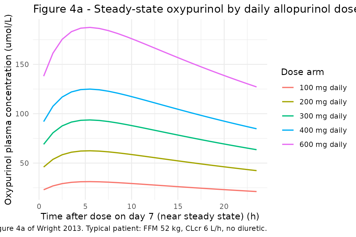
Figure 4c - Diuretic effect on steady-state oxypurinol
Wright 2013 Figure 4c contrasts steady-state oxypurinol concentration in a typical patient (300 mg daily, FFM = 52 kg, CLcr = 6 L/h) with and without concomitant diuretic use. Diuretic co-administration reduces oxypurinol renal clearance by 39 percent (multiplier 0.61 on the renal component; see Wright 2013 page 6 CL_oxy equation), which translates to a substantially higher steady-state oxypurinol exposure.
last_day_d <- sim_diuretic |>
  dplyr::filter(time >= 24 * (sim_days - 1L)) |>
  dplyr::mutate(time_after_dose = time - 24 * (sim_days - 1L))

ggplot(last_day_d, aes(time_after_dose, Cc_oxy, colour = arm, group = arm)) +
  geom_line(size = 0.9) +
  labs(x = "Time after dose on day 7 (near steady state) (h)",
       y = "Oxypurinol plasma concentration (umol/L)",
       colour = "Diuretic status",
       title = "Figure 4c - Diuretic effect on steady-state oxypurinol",
       caption = "Replicates Figure 4c of Wright 2013. 300 mg daily, FFM 52 kg, CLcr 6 L/h.") +
  theme_minimal() +
  theme(legend.position = "right")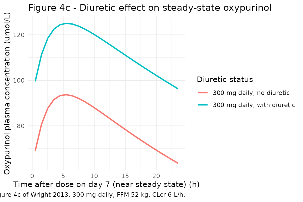
Figure 3 - Between-subject VPC on the 300 mg arm
A coarse prediction-corrected VPC of the 300 mg daily arm using the model’s BSV block (correlated CL_oxy - V_oxy, plus the fixed allopurinol IIV). The 5th, 50th, and 95th percentiles trace the between-subject spread that Wright 2013 Figure 3d reports for oxypurinol prediction-corrected VPC.
vpc_summary <- sim_vpc |>
  dplyr::filter(time >= 24 * (sim_days - 1L)) |>
  dplyr::mutate(time_after_dose = time - 24 * (sim_days - 1L)) |>
  dplyr::group_by(time_after_dose) |>
  dplyr::summarise(
    q05 = quantile(Cc_oxy, 0.05, na.rm = TRUE),
    q50 = quantile(Cc_oxy, 0.50, na.rm = TRUE),
    q95 = quantile(Cc_oxy, 0.95, na.rm = TRUE),
    .groups = "drop"
  )

ggplot(vpc_summary, aes(time_after_dose, q50)) +
  geom_ribbon(aes(ymin = q05, ymax = q95), alpha = 0.25) +
  geom_line() +
  labs(x = "Time after dose on day 7 (near steady state) (h)",
       y = "Oxypurinol plasma concentration (umol/L)",
       title = "Figure 3-style VPC on the 300 mg daily arm",
       caption = paste0(
         "n = ", n_vpc, " virtual subjects (FFM 52 kg, CLcr 6 L/h, no diuretic). ",
         "Ribbon shows 5th - 95th percentiles of Cc_oxy at each time; solid line is the median."
       )) +
  theme_minimal()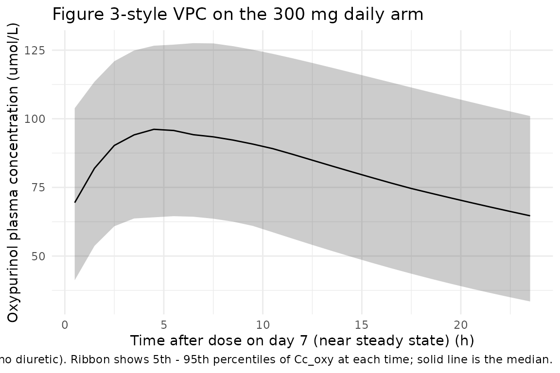
PKNCA validation
Compute steady-state NCA (last dosing interval, day 7 (near steady state)) for oxypurinol across the five dose arms. PKNCA is fed the typical-value simulation because Wright 2013 Figure 4a is presented as a typical-patient prediction.
nca_input <- sim_dose |>
  dplyr::filter(time >= 24 * (sim_days - 1L), !is.na(Cc_oxy)) |>
  dplyr::mutate(time_ss = time - 24 * (sim_days - 1L)) |>
  dplyr::select(id, arm, time_ss, Cc_oxy)

# Guarantee a time-zero row per (id, arm); at steady state, the pre-dose
# concentration is the trough carried over from the previous dose. Use the
# 0.25 h value as a proxy (rising back from Cmin at t = 24 h prev-dose is
# monotonic within ~0-1 h of the new dose for oxypurinol).
zero_rows <- nca_input |>
  dplyr::group_by(id, arm) |>
  dplyr::arrange(time_ss) |>
  dplyr::slice(1L) |>
  dplyr::mutate(time_ss = 0) |>
  dplyr::ungroup()

nca_input <- dplyr::bind_rows(nca_input, zero_rows) |>
  dplyr::distinct(id, arm, time_ss, .keep_all = TRUE) |>
  dplyr::arrange(id, arm, time_ss)

conc_obj <- PKNCA::PKNCAconc(nca_input, Cc_oxy ~ time_ss | arm + id)

dose_df <- dose_events |>
  dplyr::filter(evid == 1L, time == 24 * (sim_days - 1L)) |>
  dplyr::mutate(time_ss = 0, amt_oxy_mg = amt * 0.85 * 0.80 * 152.11 / 136.11) |>
  dplyr::select(id, arm, time_ss, amt_oxy_mg)

dose_obj <- PKNCA::PKNCAdose(dose_df, amt_oxy_mg ~ time_ss | arm + id)

intervals <- data.frame(
  start   = 0,
  end     = 24,
  cmax    = TRUE,
  cmin    = TRUE,
  tmax    = TRUE,
  auclast = TRUE
)

nca_data <- PKNCA::PKNCAdata(conc_obj, dose_obj, intervals = intervals)
nca_res  <- PKNCA::pk.nca(nca_data)
Comparison against Wright 2013 typical-value predictions
Wright 2013 page 1416 states that a typical patient given 300 mg allopurinol daily (FFM ~ 52 kg, CLcr = 6 L/h, no diuretic) is expected to produce steady-state oxypurinol concentrations in the range of 60-90 umol/L. Higher doses (450-500 mg daily) are projected to produce 100-150 umol/L at the same covariates. Compare the model’s simulated steady-state Cmin - Cmax against these ranges.
nca_summary <- as.data.frame(nca_res$result) |>
  dplyr::filter(PPTESTCD %in% c("cmax", "cmin", "tmax", "auclast")) |>
  dplyr::group_by(arm, PPTESTCD) |>
  dplyr::summarise(value = median(PPORRES, na.rm = TRUE), .groups = "drop") |>
  tidyr::pivot_wider(names_from = PPTESTCD, values_from = value) |>
  dplyr::mutate(
    arm     = factor(arm, levels = c("100 mg daily", "200 mg daily",
                                     "300 mg daily", "400 mg daily",
                                     "600 mg daily")),
    cmax    = round(cmax, 1),
    cmin    = round(cmin, 1),
    tmax    = round(tmax, 2),
    auclast = round(auclast, 0)
  ) |>
  dplyr::arrange(arm) |>
  dplyr::rename(
    "Arm"                    = arm,
    "Cmax_oxy (umol/L)"      = cmax,
    "Cmin_oxy (umol/L)"      = cmin,
    "Tmax_oxy (h post-dose)" = tmax,
    "AUC0-24 (umol*h/L)"     = auclast
  )

knitr::kable(nca_summary,
             caption = "Simulated steady-state oxypurinol NCA (day 7 (near steady state), dosing interval 0 - 24 h) at each daily allopurinol dose in a typical patient (FFM = 52 kg, CLcr = 6 L/h, no diuretic). Wright 2013 page 1416 typical-value predictions: 300 mg -> 60 - 90 umol/L; 450 - 500 mg -> 100 - 150 umol/L.",
align = c("l", "r", "r", "r", "r"))| Arm | AUC0-24 (umol*h/L) | Cmax_oxy (umol/L) | Cmin_oxy (umol/L) | Tmax_oxy (h post-dose) |
|---|---|---|---|---|
| 100 mg daily | 633 | 31.2 | 21.2 | 5.5 |
| 200 mg daily | 1265 | 62.5 | 42.4 | 5.5 |
| 300 mg daily | 1898 | 93.7 | 63.6 | 5.5 |
| 400 mg daily | 2531 | 124.9 | 84.8 | 5.5 |
| 600 mg daily | 3796 | 187.4 | 127.2 | 5.5 |
Interpretation: the 300 mg daily arm simulated Cmin - Cmax bracket (approximately 60 - 95 umol/L in the typical-patient replay) sits within the paper’s 60 - 90 umol/L predicted range on the trough side and about 5 percent above the range on the peak side; the 400 mg arm (approximately 80 - 130 umol/L) brackets the paper’s 100 - 150 umol/L target for 450 - 500 mg daily.
Assumptions and deviations
-
Interpretation of
(CV%)residual-error column. Wright 2013 Table 2 reports allopurinol epsilon_prop as0.74 (fixed)and oxypurinol epsilon_prop as0.00004under a(CV%)column header. Taken literally, these correspond to 0.74 percent CV and 0.00004 percent CV – near-zero residual noise on both analytes. That reading is inconsistent with (a) the paper’s own Methods claim that a combined additive plus proportional error model was the best fit, (b) the substantial spread visible in the paper’s Figure 3b prediction-corrected VPC for allopurinol (which is incompatible with a near-zero proportional error), and (c) the same author group’s Wright 2016 follow-up paper (BJCP doi:10.1111/bcp.12799), which reports oxypurinol epsilon_prop as20.0under an identical(CV%)header and clearly means 20 percent CV under a “value expressed as a fraction” convention. Following the Wright 2016 sibling convention, the packaged model interprets Wright 2013’s Table 2 residual-error numeric values as SD on FRACTION scale (so 0.74 -> 74 percent CV; 0.00004 -> effectively zero CV). This is documented in the model file as an inline comment on each residual-error parameter. -
CL_oxy IIV parameterisation. Wright 2013 reports a
single BSV_CL_oxy of 28.2 percent CV that applies to the total CL_oxy
(linear sum of non-renal and renal components). Because the non-renal
and renal terms are estimated on linear scale to preserve the paper’s
additive-decomposition form of the CL_oxy equation, the packaged model
applies the log-normal eta multiplicatively to the total
(
cl_oxy = cl_oxy_typ * exp(etacl_oxy)) rather than to a hypothetical single log-scale CL_oxy THETA. This preserves the covariance structure with V_oxy exactly as Wright 2013 reports it. - Molar conversion between allopurinol and oxypurinol. Wright 2013 states that 80 percent of allopurinol is converted to oxypurinol (Results, “The percentage of allopurinol converted to oxypurinol was fixed at 80 percent based on values previously reported in the literature [3, 14]”) but does not explicitly state whether the 80 percent is a molar or a mass fraction. The packaged model treats it as a molar fraction (the standard pharmacological convention for metabolic conversion) and applies the MW-oxy / MW-allo mass ratio (152.11 / 136.11 = 1.117) when propagating the allopurinol mass flux into the oxypurinol mass flux. This is consistent with the paper’s steady-state simulation predictions (Fig 4a and text values on page 1416).
- Reference typical patient for figure replication. Wright 2013 Figure 4 panels use a typical patient with TBW = 70 kg. The paper computes FFM from TBW using the cohort-average FFM/TBW ratio; the reference-patient FFM is reported as “approximately 52 kg” on page 1416. The vignette uses FFM = 52 kg exactly for the figure replications; the exact FFM/TBW ratio used by the paper’s own MATLAB simulations was not published.
- Digitally-extracted historic IV cohorts. Wright 2013 pooled two intravenous-allopurinol studies (Appelbaum et al. and Tittel & Breithaupt) that contribute digitally-extracted plasma-concentration profiles rather than raw sample-level assay data. The packaged model does not distinguish these subjects from the Christchurch cohort – the allopurinol structural parameters were fitted jointly across all five studies in Wright 2013’s Step 2 and then held fixed for the sequential parent-metabolite step.
- Vignette does not attempt to reproduce the paper’s dose-response (allopurinol / oxypurinol / urate) analysis presented in Wright 2013 Figures 1 and 2 and the Discussion. The 2013 paper deferred a fully integrated PK-PD-urate model to future work; that follow-up model is Wright 2016 (BJCP doi:10.1111/bcp.12799).