Lithium (Jin 2022) • nlmixr2lib

Model and source

Citation: Jin Z-b, Wu Z, Cui Y-f, Liu X-p, Liang H-b, You J-y, Wang C-y. Population Pharmacokinetics and Dosing Regimen of Lithium in Chinese Patients With Bipolar Disorder. Front Pharmacol. 2022;13:913935. doi:10.3389/fphar.2022.913935. PMC9289112. Parameter estimates are in Table 2; the final covariate model is Results Equations 8-10.
Description: One-compartment population pharmacokinetic model with first-order absorption (ka fixed) and first-order elimination for lithium in 268 Chinese patients with bipolar disorder on lithium carbonate maintenance therapy (trough therapeutic-drug-monitoring samples), from Jin 2022. Apparent clearance CL/F scales as a power of total daily lithium carbonate dose (centred on 600 mg/day), body weight (62 kg) and Cockcroft-Gault creatinine clearance (116 mL/min). Doses are in mmol of lithium ion (1 mg lithium carbonate = 2 / 73.89 mmol Li) and concentrations in mmol/L.
Article: https://doi.org/10.3389/fphar.2022.913935 (PMC9289112, open access)

Population

Jin 2022 pooled 476 trough serum lithium concentrations from 268 Chinese patients with bipolar disorder on lithium carbonate maintenance treatment at the Affiliated Xuzhou Eastern Hospital of Xuzhou Medical University between September 2016 and August 2021 (Methods 2.1, Table 1). Two thirds were women (179, 66.8%); median age was 31.0 years (range 13.0-77.0), and 241 (89.9%) were adults older than 16 years. Median body weight was 62.0 kg (35.0-110), the median total daily dose 600 mg lithium carbonate (150-1500), and median Cockcroft-Gault creatinine clearance 116 mL/min (61.7-226). 76.1% of patients took sustained-release tablets and 23.9% ordinary tablets. Every sample was drawn before the morning dose; patients taking diuretics, renin-angiotensin-system antagonists or serotonergic drugs were excluded.

The same information is available programmatically via rxode2::rxode(readModelDb("Jin_2022_lithium"))$population.

Source trace

Every ini() value carries an in-file comment in inst/modeldb/specificDrugs/Jin_2022_lithium.R. The table collects them.

Equation / parameter	Value	Source location
Structure: depot -> central, first-order absorption and elimination	n/a	Methods 2.2.1; Results 3.2
`lka`	fixed(log(0.293 1/h))	Table 2, Ka ‘[fixed]’; Equation 10; Methods 2.2.1
`lcl`	log(0.909 L/h)	Table 2, CL; Equation 8
`lvc`	log(10.9 L)	Table 2, V; Equation 9
`e_dose_lithium_cl`	0.354	Table 2, ‘TDD on CL’; Equation 8 `(TDD/600)^0.354`
`e_wt_cl`	0.33	Table 2, ‘WT on CL’; Equation 8 `(WT/62)^0.33`
`e_crcl_cl`	0.186	Table 2, ‘CRCL on CL’; Equation 8 `(CRCL/116)^0.186`
`etalcl`	0.027 (16.4%)	Equation 8 exponent; Table 2, BSV CL
`etalvc`	0.162 (40.2%)	Equation 9 exponent; Table 2, BSV V
`addSd`	sqrt(0.0218) = 0.148 mmol/L	Table 2, additive error (read as a variance; see below)
`Cc ~ add(addSd)`	n/a	Table 2 (only an additive term is reported); Methods 2.2.1
CRCL equation	Cockcroft-Gault, Scr in umol/L, divisor 0.818	Table 1 footnote

Equations 8 and 9 print the exponents e^0.027 and e^0.162, which are the raw omega^2 estimates: Table 2 reports the same BSV as 16.4% and 40.2%, and sqrt(0.027) = 0.164, sqrt(0.162) = 0.402. They are used directly as the eta variances.

Dose unit

Lithium carbonate (Li2CO3, 73.89 g/mol) carries two lithium ions, so 1 mg lithium carbonate = 2 / 73.89 = 0.02707 mmol Li. The paper reports concentrations in mmol/L and clearance in L/h without printing the conversion; the model doses in mmol of lithium ion. The covariate DOSE_LITHIUM_CARBONATE_MGD keeps the clinical unit (mg of the salt per day) because Equation 8 centres it on 600 mg.

mg_li2co3_to_mmol_li <- function(mg) mg * 2 / 73.89

# Typical CL/F (L/h) from Equation 8.
cl_eq8 <- function(tdd, wt, crcl) {
  0.909 * (tdd / 600)^0.354 * (wt / 62)^0.33 * (crcl / 116)^0.186
}

# Twice-daily oral dosing for `days` days, one trough (or a profile) after it.
# `tdd` is the value given to the CL/F covariate, which may differ from the
# simulated dose (see the Figure 3 section).
make_events <- function(cohort, obs_times, tau = 12, days = 7) {
  dose_times <- seq(0, days * 24 - tau, by = tau)
  doses <- tidyr::crossing(cohort, time = dose_times) |>
    mutate(evid = 1L, cmt = "depot", amt = mg_li2co3_to_mmol_li(dose_mgd * tau / 24))
  obs <- tidyr::crossing(cohort, time = obs_times) |>
    mutate(evid = 0L, cmt = "central", amt = 0)
  bind_rows(doses, obs) |>
    arrange(id, time, desc(evid)) |>
    relocate(id, time, evid, amt, cmt)
}

Typical clearance claims in the text

The Results and Discussion state three typical-value consequences of Equation 8. They follow in closed form from the printed parameters.

cl_ref <- cl_eq8(600, 62, 116)
cl_crcl_drop <- 1 - cl_eq8(600, 62, 30) / cl_eq8(600, 62, 120)
cl_50 <- cl_eq8(600, 50, 116)
cl_100 <- cl_eq8(600, 100, 116)

tibble(
  Claim = c(
    "CL/F, 62 kg, CRCL 116 mL/min, 600 mg/day (L/h)",
    "Fall in CL/F, CRCL 120 -> 30 mL/min (%)",
    "CL/F at 50 kg (L/h)",
    "CL/F at 100 kg (L/h)",
    "Rise in CL/F, 50 -> 100 kg (%)"
  ),
  Paper = c(0.909, 23, 0.83, 1.06, 28),
  Model = c(cl_ref, 100 * cl_crcl_drop, cl_50, cl_100, 100 * (cl_100 / cl_50 - 1))
) |>
  knitr::kable(digits = 3)

Claim	Paper	Model
CL/F, 62 kg, CRCL 116 mL/min, 600 mg/day (L/h)	0.909	0.909
Fall in CL/F, CRCL 120 -> 30 mL/min (%)	23.000	22.729
CL/F at 50 kg (L/h)	0.830	0.847
CL/F at 100 kg (L/h)	1.060	1.064
Rise in CL/F, 50 -> 100 kg (%)	28.000	25.701


# Closed form, no simulation noise. A mis-transcribed exponent moves these
# by far more than the tolerances.
stopifnot(
  abs(cl_ref - 0.909) < 1e-9,
  abs(100 * cl_crcl_drop - 23) < 0.5,
  abs(cl_100 - 1.06) < 0.01
)

The 23% fall with renal function and the 1.06 L/h at 100 kg reproduce exactly. At 50 kg the model gives 0.847 L/h, not the 0.83 L/h quoted in the Discussion, so the quoted 28% rise is 26% under Equation 8 (2^0.33 = 1.257 for any doubling of weight). The dose and renal-function factors cancel in the ratio, so 1.06 / 0.83 = 1.28 cannot arise from Equation 8 under any covariate values; the 0.83 appears to be a slip in the Discussion.

Residual error scale

Table 2 prints the residual as ‘Additive error (mmol/L) 0.0218’, with 20% epsilon shrinkage. The unit suggests an SD, but the Equations print the omegas as raw variances, so 0.0218 may equally be the NONMEM $SIGMA variance (SD 0.148 mmol/L). The goodness-of-fit plot separates the two: the spread of observations about the individual predictions is roughly sigma * (1 - shrinkage). The maintainers digitised Figure 1A (observed vs individual predicted concentration) from the 300-dpi article page by locating every marker pixel, calibrating the axes on the identity line (fitted slope 0.998, intercept 0.001). The vertical scatter about that line has an SD of 0.13-0.15 mmol/L across the prediction range (marker size included).

ruv <- tibble(
  Reading = c("0.0218 is the SD", "0.0218 is the variance"),
  `Residual SD (mmol/L)` = c(0.0218, sqrt(0.0218)),
  `Expected IPRED scatter (mmol/L)` = c(0.0218, sqrt(0.0218)) * (1 - 0.20),
  `Figure 1A scatter (mmol/L)` = 0.14
)
knitr::kable(ruv, digits = 3)

Reading	Residual SD (mmol/L)	Expected IPRED scatter (mmol/L)	Figure 1A scatter (mmol/L)
0.0218 is the SD	0.022	0.017	0.14
0.0218 is the variance	0.148	0.118	0.14

Read as an SD, the observations in Figure 1A would lie within about +/-0.04 mmol/L of the identity line; they spread over about +/-0.3 mmol/L. The variance reading is adopted and the model uses addSd = sqrt(0.0218). Figure 3 (below) gives independent support: its 250 mg boxes have lower whiskers at 0 mmol/L in every panel, which only an additive error of this size produces.

Steady-state troughs by weight, renal function and dose (Figure 3)

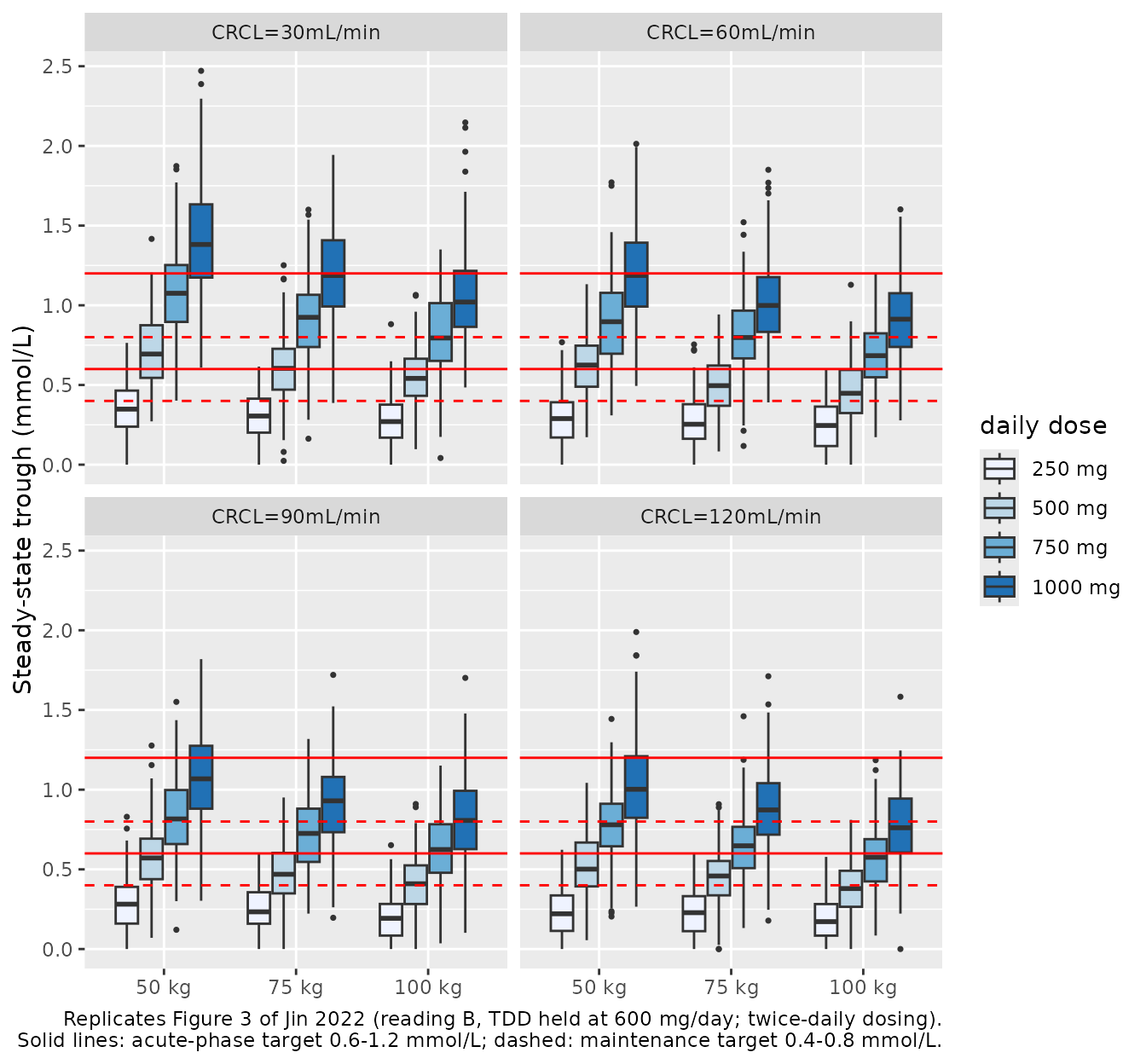
Jin 2022 simulated steady-state troughs after 7 days of dosing for daily doses of 250-1000 mg lithium carbonate, body weights of 50, 75 and 100 kg and creatinine clearances of 30, 60, 90 and 120 mL/min (Methods 2.4, Results 3.4, Figure 3). The paper does not state the dosing frequency; twice-daily dosing is used here (the trough is taken 12 h after the 14th dose, at 168 h).

The Figure 3 box medians were digitised by the maintainers from the 300-dpi article page by locating each box’s median bar; the axis calibration was checked on the red target lines, which it places within 0.003 mmol/L of 0.4, 0.6, 0.8 and 1.2.

fig3 <- tidyr::expand_grid(
  CRCL = c(30, 60, 90, 120),
  WT = c(50, 75, 100),
  dose_mgd = c(250, 500, 750, 1000)
) |>
  mutate(fig_median = c(
    0.399, 0.768, 1.103, 1.365, 0.332, 0.665, 0.950, 1.210, 0.279, 0.599, 0.861, 1.094,
    0.328, 0.690, 0.961, 1.201, 0.279, 0.588, 0.816, 1.045, 0.239, 0.499, 0.748, 0.948,
    0.311, 0.615, 0.888, 1.108, 0.247, 0.515, 0.762, 0.964, 0.240, 0.480, 0.691, 0.891,
    0.286, 0.586, 0.833, 1.033, 0.240, 0.491, 0.722, 0.913, 0.224, 0.440, 0.660, 0.842
  ))

The Figure 3 medians rise in proportion to the dose: within each weight and renal-function panel, the 1000 mg median is about 3.8 times the 250 mg median. Equation 8 makes CL/F rise as TDD^0.354, so the printed model predicts troughs that rise only as TDD^0.646, a ratio of 4^0.646 = 2.45. Figure 3 therefore appears to have been simulated with the total-daily-dose covariate held at the value in the original dataset (“simulations were performed using the initial dataset”, Methods 2.4) while the simulated doses changed. Both readings are simulated: (A) the model as printed, with DOSE_LITHIUM_CARBONATE_MGD equal to the simulated daily dose; and (B) DOSE_LITHIUM_CARBONATE_MGD held at the 600 mg/day reference. 200 virtual patients per scenario.

mod <- readModelDb("Jin_2022_lithium")
n_per <- 200
scen <- fig3 |>
  select(CRCL, WT, dose_mgd) |>
  mutate(scenario = row_number())
cohort_fig3 <- bind_rows(
  scen |> mutate(reading = "A: printed (TDD = dose)", DOSE_LITHIUM_CARBONATE_MGD = dose_mgd),
  scen |> mutate(reading = "B: TDD held at 600 mg/day", DOSE_LITHIUM_CARBONATE_MGD = 600)
) |>
  slice(rep(seq_len(n()), each = n_per)) |>
  mutate(id = row_number())
events_fig3 <- make_events(cohort_fig3, obs_times = 168)

rxode2::rxSetSeed(20220704)
sim_fig3 <- rxode2::rxSolve(
  mod,
  events = events_fig3,
  keep = c("reading", "scenario", "dose_mgd", "WT", "CRCL")
) |>
  as.data.frame() |>
  filter(time == 168) |>
  mutate(trough = pmax(sim, 0))
#> [====|====|====|====|====|====|====|====|====|====] 0:00:09
stopifnot(nrow(sim_fig3) == nrow(cohort_fig3))

sim_fig3 |>
  mutate(
    panel = factor(paste0("CRCL=", CRCL, "mL/min"), levels = paste0("CRCL=", c(30, 60, 90, 120), "mL/min")),
    `daily dose` = factor(paste(dose_mgd, "mg"), levels = paste(c(250, 500, 750, 1000), "mg"))
  ) |>
  filter(reading == "B: TDD held at 600 mg/day") |>
  ggplot(aes(factor(paste(WT, "kg"), levels = paste(c(50, 75, 100), "kg")), trough, fill = `daily dose`)) +
  geom_boxplot(outlier.size = 0.6) +
  geom_hline(yintercept = c(0.6, 1.2), colour = "red") +
  geom_hline(yintercept = c(0.4, 0.8), colour = "red", linetype = "dashed") +
  scale_fill_brewer(palette = "Blues") +
  facet_wrap(~panel) +
  labs(
    x = NULL, y = "Steady-state trough (mmol/L)",
    caption = paste(
      "Replicates Figure 3 of Jin 2022 (reading B, TDD held at 600 mg/day; twice-daily dosing).",
      "Solid lines: acute-phase target 0.6-1.2 mmol/L; dashed: maintenance target 0.4-0.8 mmol/L.",
      sep = "\n"
    )
  )

med_fig3 <- sim_fig3 |>
  group_by(reading, CRCL, WT, dose_mgd) |>
  summarise(sim_median = median(trough), .groups = "drop") |>
  inner_join(fig3, by = c("CRCL", "WT", "dose_mgd")) |>
  mutate(pct_diff = 100 * (sim_median / fig_median - 1))
stopifnot(nrow(med_fig3) == 2 * nrow(fig3))

dose_ratio <- med_fig3 |>
  group_by(reading, CRCL, WT) |>
  summarise(
    sim = sim_median[dose_mgd == 1000] / sim_median[dose_mgd == 250],
    fig = fig_median[dose_mgd == 1000] / fig_median[dose_mgd == 250],
    .groups = "drop"
  )

summary_fig3 <- med_fig3 |>
  group_by(reading) |>
  summarise(
    median_pct_diff = median(pct_diff),
    p90_abs_pct_diff = quantile(abs(pct_diff), 0.9),
    .groups = "drop"
  ) |>
  inner_join(
    dose_ratio |>
      group_by(reading) |>
      summarise(sim_ratio = median(sim), fig_ratio = median(fig), .groups = "drop"),
    by = "reading"
  )
summary_fig3 |>
  rename(
    "Reading" = reading,
    "Median % difference vs Figure 3" = median_pct_diff,
    "90th pct of |% difference|" = p90_abs_pct_diff,
    "Simulated 1000/250 mg ratio" = sim_ratio,
    "Figure 3 1000/250 mg ratio" = fig_ratio
  ) |>
  knitr::kable(digits = 2)

Reading	Median % difference vs Figure 3	90th pct of \|% difference\|	Simulated 1000/250 mg ratio	Figure 3 1000/250 mg ratio
A: printed (TDD = dose)	-10.91	37.36	2.10	3.73
B: TDD held at 600 mg/day	-8.06	14.51	3.95	3.73


pct_b <- med_fig3$pct_diff[med_fig3$reading == "B: TDD held at 600 mg/day"]
ratio_a <- dose_ratio$sim[dose_ratio$reading == "A: printed (TDD = dose)"]
ratio_b <- dose_ratio$sim[dose_ratio$reading == "B: TDD held at 600 mg/day"]
stopifnot(
  # Figure 3 itself is dose-proportional (digitised, no simulation noise).
  median(dose_ratio$fig) > 3.4,
  # Reading B: the 48 medians are each from 200 subjects (sampling SE about
  # 3%). Closed-form typical troughs sit 8% below the figure on average; the
  # remaining offset is the unstated dosing frequency (three-times-daily
  # dosing would put them 5% above). A wrong CL, V, exponent or mg -> mmol
  # factor moves every cell by tens of percent.
  abs(median(pct_b)) < 15,
  quantile(abs(pct_b), 0.9) < 25,
  # The dose proportionality separates the readings: about 4.0 for B and
  # 2.1 for A (closed form), against 3.8 in the figure.
  abs(median(ratio_b) / median(dose_ratio$fig) - 1) < 0.15,
  median(ratio_a) < 2.7
)

Reading B reproduces the Figure 3 medians to within about 8% on average (simulated slightly lower; the unstated dosing frequency accounts for an offset of this size), including their proportionality to dose. Reading A, the model as printed, gives troughs that are too high at 250 mg and too low at 1000 mg relative to the figure:

med_fig3 |>
  filter(CRCL %in% c(30, 120)) |>
  select(reading, CRCL, WT, dose_mgd, fig_median, sim_median) |>
  pivot_wider(names_from = reading, values_from = sim_median) |>
  rename(
    "CRCL (mL/min)" = CRCL,
    "WT (kg)" = WT,
    "Daily dose (mg)" = dose_mgd,
    "Figure 3 median (mmol/L)" = fig_median
  ) |>
  knitr::kable(digits = 2, caption = "Median steady-state trough, CRCL 30 and 120 mL/min panels.")

Median steady-state trough, CRCL 30 and 120 mL/min panels.
CRCL (mL/min)	WT (kg)	Daily dose (mg)	Figure 3 median (mmol/L)	A: printed (TDD = dose)	B: TDD held at 600 mg/day
30	50	250	0.40	0.52	0.35
30	50	500	0.77	0.76	0.69
30	50	750	1.10	0.97	1.08
30	50	1000	1.36	1.10	1.38
30	75	250	0.33	0.42	0.31
30	75	500	0.66	0.66	0.60
30	75	750	0.95	0.78	0.92
30	75	1000	1.21	0.98	1.19
30	100	250	0.28	0.39	0.27
30	100	500	0.60	0.61	0.54
30	100	750	0.86	0.74	0.79
30	100	1000	1.09	0.87	1.02
120	50	250	0.29	0.38	0.22
120	50	500	0.59	0.56	0.50
120	50	750	0.83	0.73	0.78
120	50	1000	1.03	0.79	1.00
120	75	250	0.24	0.34	0.23
120	75	500	0.49	0.46	0.46
120	75	750	0.72	0.58	0.65
120	75	1000	0.91	0.67	0.87
120	100	250	0.22	0.31	0.17
120	100	500	0.44	0.42	0.38
120	100	750	0.66	0.53	0.58
120	100	1000	0.84	0.59	0.76

The shipped model keeps Equation 8 as printed (reading A): the dose effect on CL/F is an estimated parameter with 12% RSE and a bootstrap interval excluding zero, and the Discussion interprets it as nonlinear renal excretion. Reading B describes only how Figure 3 and its dosing recommendations were produced. To reproduce them, set DOSE_LITHIUM_CARBONATE_MGD = 600 while dosing the regimen of interest.

Truncation at zero

Figure 3 shows lower whiskers at 0 mmol/L for every 250 mg box. With the shipped residual SD (0.148 mmol/L), a share of simulated 250 mg troughs falls below zero and is truncated; with an SD of 0.0218 almost none would.

cohort_250 <- scen |>
  filter(dose_mgd == 250) |>
  mutate(DOSE_LITHIUM_CARBONATE_MGD = 600) |>
  slice(rep(seq_len(n()), each = n_per)) |>
  mutate(id = row_number())
events_250 <- make_events(cohort_250, obs_times = 168)
mod_sd_reading <- rxode2::rxode(mod) |> rxode2::ini(addSd = 0.0218)
#> ℹ change initial estimate of `addSd` to `0.0218`
rxode2::rxSetSeed(20220705)
sim_250 <- bind_rows(
  rxode2::rxSolve(mod, events = events_250) |>
    as.data.frame() |>
    mutate(reading = "addSd = sqrt(0.0218) (shipped)"),
  rxode2::rxSolve(mod_sd_reading, events = events_250) |>
    as.data.frame() |>
    mutate(reading = "addSd = 0.0218")
) |>
  filter(time == 168)
trunc_share <- sim_250 |>
  group_by(reading) |>
  summarise(pct_below_zero = 100 * mean(sim < 0), .groups = "drop")
knitr::kable(trunc_share, digits = 1)

reading	pct_below_zero
addSd = 0.0218	0.0
addSd = sqrt(0.0218) (shipped)	5.5

stopifnot(
  # 2400 subjects per reading: a share of several percent against well under
  # 1%; the SE of either share is below 0.6 percentage points.
  trunc_share$pct_below_zero[trunc_share$reading == "addSd = sqrt(0.0218) (shipped)"] > 3,
  trunc_share$pct_below_zero[trunc_share$reading == "addSd = 0.0218"] < 1
)

Steady-state NCA (model as printed)

A typical patient (62 kg, CRCL 116 mL/min) takes each daily dose twice daily for 7 days, with DOSE_LITHIUM_CARBONATE_MGD equal to the dose. The paper reports no NCA, so the check is that the steady-state AUC over a dosing interval equals the dose divided by CL/F: CL/F is monotone in its eta, so the median AUC equals the dose over the typical CL/F.

cohort_nca <- tibble(dose_mgd = c(250, 500, 750, 1000)) |>
  mutate(
    WT = 62, CRCL = 116, DOSE_LITHIUM_CARBONATE_MGD = dose_mgd,
    treatment = paste(dose_mgd, "mg/day")
  ) |>
  slice(rep(seq_len(n()), each = n_per)) |>
  mutate(id = row_number())
events_nca <- make_events(cohort_nca, obs_times = c(0, seq(156, 168, by = 0.25)))
rxode2::rxSetSeed(20220706)
sim_nca <- rxode2::rxSolve(mod, events = events_nca, keep = c("treatment", "dose_mgd")) |>
  as.data.frame()

conc_nca <- sim_nca |>
  filter(!is.na(Cc)) |>
  mutate(Cc = pmax(Cc, 0)) |>
  select(id, time, Cc, treatment)
dose_nca <- events_nca |>
  filter(evid == 1) |>
  select(id, time, amt, treatment)
nca <- PKNCA::pk.nca(
  PKNCA::PKNCAdata(
    PKNCA::PKNCAconc(conc_nca, Cc ~ time | treatment + id),
    PKNCA::PKNCAdose(dose_nca, amt ~ time | treatment + id),
    intervals = data.frame(
      start = 156, end = 168,
      cmax = TRUE, cmin = TRUE, cav = TRUE, auclast = TRUE
    )
  )
)
nca_df <- as.data.frame(nca)

nca_df |>
  filter(PPTESTCD %in% c("cmax", "cmin", "cav", "auclast")) |>
  group_by(treatment, PPTESTCD) |>
  summarise(median = median(PPORRES), .groups = "drop") |>
  pivot_wider(names_from = PPTESTCD, values_from = median) |>
  mutate(treatment = factor(treatment, levels = paste(c(250, 500, 750, 1000), "mg/day"))) |>
  arrange(treatment) |>
  rename(
    "Daily dose" = treatment,
    "Cmax (mmol/L)" = cmax,
    "Cmin (mmol/L)" = cmin,
    "Cav (mmol/L)" = cav,
    "AUCtau (mmol*h/L)" = auclast
  ) |>
  knitr::kable(digits = 3, caption = "Median steady-state exposure, 62 kg, CRCL 116 mL/min, twice daily.")

Median steady-state exposure, 62 kg, CRCL 116 mL/min, twice daily.
Daily dose	AUCtau (mmol*h/L)	Cav (mmol/L)	Cmax (mmol/L)	Cmin (mmol/L)
250 mg/day	5.116	0.426	0.472	0.347
500 mg/day	7.877	0.656	0.754	0.501
750 mg/day	10.224	0.852	0.999	0.632
1000 mg/day	12.351	1.029	1.225	0.737

auc_chk <- nca_df |>
  filter(PPTESTCD == "auclast") |>
  inner_join(distinct(cohort_nca, id, dose_mgd), by = "id") |>
  group_by(dose_mgd) |>
  summarise(sim = median(PPORRES), .groups = "drop") |>
  mutate(
    expected = mg_li2co3_to_mmol_li(dose_mgd / 2) / cl_eq8(dose_mgd, 62, 116),
    pct_diff = 100 * (sim / expected - 1)
  )
knitr::kable(auc_chk, digits = 3)

dose_mgd	sim	expected	pct_diff
250	5.116	5.074	0.824
500	7.877	7.941	-0.804
750	10.224	10.318	-0.910
1000	12.351	12.426	-0.598

# The median of 200 subjects carries a sampling SE of about 1.5% (CL IIV
# 16.4%); 7 days is more than 20 half-lives, and the 0.25-h trapezoid error
# is under 0.5%. A wrong dose unit or CL/F moves this by tens of percent.
stopifnot(nrow(auc_chk) == 4, max(abs(auc_chk$pct_diff)) < 6)

Assumptions and deviations

Figure 3 simulation. The Figure 3 medians, and the dosing recommendations drawn from them (Results 3.4, Discussion), are proportional to dose and are reproduced only with the total-daily-dose covariate held fixed (reading B, 600 mg/day). The model ships Equation 8 as printed. Under the printed model the recommended regimens still mostly land in their windows (for 100 kg and CRCL 120 mL/min, 750 mg/day given twice daily gives a median trough of about 0.53 mmol/L and 1000 mg/day about 0.59 mmol/L), but 1000 mg/day then sits at the lower edge of the 0.6-1.2 mmol/L acute range rather than inside it.
Dosing frequency. Not stated for the simulations or the cohort; twice-daily dosing is assumed for Figure 3 and the NCA.
Residual error. Table 2’s 0.0218 is read as the additive-error variance (SD 0.148 mmol/L), from the Figure 1A scatter and the Figure 3 whiskers; see ‘Residual error scale’. The model has no proportional term because none is reported.
Dose unit. Doses in mmol of lithium ion, 1 mg Li2CO3 = 2 / 73.89 mmol; not printed in the paper but required by mmol/L concentrations and L/h clearance.
Absorption. Ka was fixed at 0.293 1/h ‘based on published data’ without a citation; the sensitivity analysis (0.146-0.586 1/h) moved CL/F between 0.825 and 0.959 L/h. The same ka applies to sustained-release and ordinary tablets; formulation was not a covariate.
50 kg clearance. The Discussion’s 0.83 L/h at 50 kg is not reproduced (0.847 L/h under Equation 8); its 1.06 L/h at 100 kg and the 23% fall at CRCL 30 mL/min are.
Figure 2 (VPC). Not replicated: it plots the observed troughs against time since the start of therapy in days, which needs the individual dosing histories.
Covariates not retained. Sex was tested and not retained (no coefficient reported); it is recorded in covariatesDataExcluded.
Extrapolation. Figure 3 uses CRCL down to 30 mL/min, below the observed minimum of 61.7 mL/min.
No erratum or correction notice for this article was found in Europe PMC (PMID 35860024) as of 2026-10-02. The supplementary material is a Word copy of Tables 1 and 2 with the same values.