Enrofloxacin and ciprofloxacin PBPK in pigs (Zhou 2021b)
Source:vignettes/articles/Zhou_2021b_enrofloxacin_pig_pbpk.Rmd
Zhou_2021b_enrofloxacin_pig_pbpk.RmdModel and source
- Citation: Zhou K, Liu A, Ma W, Sun L, Mi K, Xu X, Algharib SA, Xie S, Huang L. Apply a Physiologically Based Pharmacokinetic Model to Promote the Development of Enrofloxacin Granules: Predict Withdrawal Interval and Toxicity Dose. Antibiotics (Basel). 2021;10(8):955. doi:10.3390/antibiotics10080955. Model equations transcribed from Supplementary File S2 (acslX code), which the authors adapted from Lin et al. 2016; parameter values from Supplementary Tables S7 and S8, Monte Carlo distributions from Supplementary Table S4.
- Article: https://doi.org/10.3390/antibiotics10080955
- Supplementary information (Tables S1-S8, File S2 acslX model code): https://www.mdpi.com/article/10.3390/antibiotics10080955/s1
Zhou and colleagues developed an oral enrofloxacin granule for pigs and built a physiologically based pharmacokinetic (PBPK) model to answer two regulatory questions without additional slaughter studies: the withdrawal time of the granule in edible tissues, and the oral dose at which the liver would be exposed to a hepatotoxic enrofloxacin concentration. The model has a parent (enrofloxacin) sub-model and a ciprofloxacin sub-model, because the residue marker for enrofloxacin products is enrofloxacin plus ciprofloxacin. Both sub-models have venous and arterial blood, an in-series lung and perfusion-limited liver, kidney, muscle, fat and rest-of-body compartments. Only unbound arterial drug perfuses the tissues. Enrofloxacin enters from a stomach and an intestinal lumen, is metabolised in the liver (35% of the metabolised amount forming ciprofloxacin) and is excreted renally. Ciprofloxacin is excreted renally.
The model equations come from Supplementary File S2 (acslX code, which the authors adapted from Lin et al. 2016). Parameter values come from Tables S7 (physiology) and S8 (chemical-specific), and the Monte Carlo distributions from Table S4.
mod <- readModelDb("Zhou_2021b_enrofloxacin_pig_pbpk")
mod_typ <- rxode2::zeroRe(mod)
Population
Residue depletion study (Zhou 2021 Section 4.3): 18 treated pigs and 2 controls; three treated pigs were slaughtered at each of 0.042, 0.5, 1, 2, 3 and 5 days after the last dose and muscle, fat, liver and kidney were assayed for enrofloxacin and ciprofloxacin by fluorescence HPLC (LOD = LOQ = 0.02 ug/mL; Table S2). The model was not fitted statistically. Physiological parameters are pig literature values (Table S7); the chemical-specific parameters come from Lin et al. 2016, with the absorption rate constant Ka, the ciprofloxacin urinary rate constant Kurine1C and the partition coefficients adjusted by hand to the residue data (Section 4.5). Plasma predictions were compared against an earlier plasma study by the same group (Figure S1, ref. 3). The Monte Carlo withdrawal-time analysis used 1000 virtual pigs (Section 4.7).
Twenty clinically healthy three-way hybrid pigs weighing 55 +/- 10 kg were used (Zhou 2021 Section 4.2). Eighteen pigs received the enrofloxacin granule in feed at 5 mg/kg twice daily for 5 days. Three were slaughtered at each of 0.042, 0.5, 1, 2, 3 and 5 days after the last dose, and muscle, fat, liver and kidney were assayed for enrofloxacin and ciprofloxacin (Table S2). The model’s reference body weight is the cohort mean of 55 kg (Table S7).
Source trace
| Quantity | Value | Source |
|---|---|---|
| Cardiac output QCC | 5 L/h/kg | Table S7; File S2 QCC
|
| Blood flow fractions QLC / QKC / QMC / QFC / Qrest | 0.2725 / 0.12 / 0.251 / 0.1275 / 0.229 | Table S7; File S2 (Qrest = QC - QL - QK - QM - QF) |
| Volume fractions VLC / VKC / VMC / VFC / VLuC / VBloodC / Vrest | 0.0247 / 0.004 / 0.4 / 0.32 / 0.01 / 0.06 / 0.1813 | Table S7; File S2
(Vrest = BW - sum of other volumes) |
| Venous / arterial share of blood | 0.74 / 0.26 | File S2 Vven, Vart
|
Body weight BW (WT) |
55 kg | Table S7; File S2 BW; Section 4.2 |
Gastric emptying Kst (lkst) |
2 1/h | Table S8; File S2 |
Intestinal absorption Ka (lka) |
0.55 1/h | Table S8; File S2; adjusted by hand (Section 4.5) |
Faecal elimination Kfeces (lkfec) |
0.01 1/h | Table S8; File S2 |
Enrofloxacin PCs PL / PK / PM / PF / PLu / Prest
(lkp_*) |
3.2 / 5.5 / 2.5 / 0.6 / 4.3 / 8 | Table S8; File S2 |
Ciprofloxacin PCs PL1 / PK1 / PM1 / PF1 / Prest1
(lkp_*_cipro) |
4.3 / 5.5 / 1.5 / 0.53 / 8 | Table S8; File S2 |
Hepatic metabolic rate KmC (kmet) |
0.035 1/(h kg) | Table S8; File S2 (Km = KmC*BW) |
Fraction metabolised to ciprofloxacin Frac (fm) |
0.35 | Table S8; File S2 |
Protein binding PB / PB1 (fu = 1 - PB) |
0.46 / 0.19 bound | Table S8; File S2 (CAfree = CA*(1-PB)) |
Urinary rate KurineC / Kurine1C (lcl_renal,
lcl_renal_cipro) |
0.12 / 0.35 L/h/kg | Table S8; File S2 |
| Molar conversions MWmol / MWmg / MW1 | 2.78 umol/mg / 0.36 mg/umol / 331.34 g/mol | File S2 |
| Monte Carlo SDs (12 etas) | see model file | Table S4 SD column |
| Oral input: stomach -> intestine -> liver, faecal loss | equations | File S2 RAST, RAI, RAO,
RL
|
| Blood, lung and tissue mass balances | equations | File S2 RV, RA, RALu,
RK, RM, RF,
Rrest
|
| Hepatic metabolism and ciprofloxacin formation |
Rmet = Km*AL, Rmet1 = Frac*Rmet
|
File S2 |
| Renal excretion | Rurine = Kurine*CVK |
File S2 |
| Residue marker | enrofloxacin + ciprofloxacin (C*_total) |
File S2 CLtotalmg etc.; Section 4.8 |
| Maximum residue limits | muscle 0.1, fat 0.1, liver 0.2, kidney 0.3 ug/g | Section 4.8; Table S2 |
Typical pig, 5 mg/kg twice daily for 5 days
The dosing in File S2 is PULSE(0, 12, 0.001) inside a
window from 0 to 120 h. That gives 10 doses at 0, 12, …, 108 h, each
delivered to the stomach over 0.001 h, which is treated here as a bolus.
The residue sampling times are days after the last dose, i.e. after 108
h; Figures 1-3 of the paper place the observations at about 109, 120,
132, 156 and 180 h.
wt_ref <- 55
t_last <- 108
make_events <- function(dose_mgkg, wt = wt_ref, times = seq(0, 228, by = 0.1)) {
  rxode2::et(amt = dose_mgkg * wt, cmt = "stomach", ii = 12, addl = 9) |>
    rxode2::et(times, cmt = "venous") |>
    as.data.frame() |>
    dplyr::mutate(WT = wt)
}
sim5 <- rxode2::rxSolve(mod_typ, make_events(5), returnType = "data.frame")
#> ℹ omega/sigma items treated as zero: 'etalkp_liver', 'etalkp_kidney', 'etalkp_muscle', 'etalkp_adipose', 'etalkp_liver_cipro', 'etalkp_kidney_cipro', 'etalkp_muscle_cipro', 'etalkp_adipose_cipro', 'etakmet', 'etafm', 'etalcl_renal', 'etalcl_renal_cipro'
# Zhou 2021 Table S2 (mean +/- SD, n = 3). "< LOD" rows are omitted. The
# kidney ciprofloxacin SD at 0.042 d is printed "0.0.109" and is read as 0.109.
obs <- tibble::tribble(
  ~tissue,  ~day,  ~enr,  ~enr_sd, ~cip,  ~cip_sd,
  "muscle", 0.042, 3.13,  0.111,   0.644, 0.108,
  "muscle", 0.5,   1.839, 0.076,   0.387, 0.040,
  "muscle", 1,     0.719, 0.007,   0.239, 0.010,
  "muscle", 2,     0.139, 0.027,   0.097, 0.021,
  "muscle", 3,     0.039, 0.006,   0.019, 0.003,
  "fat",    0.042, 1.183, 0.108,   0.164, 0.013,
  "fat",    0.5,   0.382, 0.040,   0.111, 0.079,
  "fat",    1,     0.178, 0.006,   0.061, 0.021,
  "fat",    2,     0.049, 0.017,   0.036, 0.011,
  "liver",  0.042, 6.817, 0.047,   2.341, 0.397,
  "liver",  0.5,   1.934, 0.054,   1.350, 0.038,
  "liver",  1,     0.692, 0.035,   0.843, 0.171,
  "liver",  2,     0.184, 0.067,   0.602, 0.234,
  "liver",  3,     0.082, 0.005,   0.124, 0.004,
  "kidney", 0.042, 6.270, 0.504,   1.604, 0.109,
  "kidney", 0.5,   2.852, 0.282,   1.160, 0.097,
  "kidney", 1,     1.301, 0.310,   1.0,   0.194,
  "kidney", 2,     0.432, 0.131,   0.292, 0.119,
  "kidney", 3,     0.221, 0.027,   0.040, 0.012
) |>
  dplyr::mutate(time = t_last + 24 * day, total = enr + cip)

tissue_cols <- c(muscle = "Cmuscle", fat = "Cadipose", liver = "Cliver", kidney = "Ckidney")
long_pred <- function(sim, suffix, analyte) {
  cols <- paste0(tissue_cols, suffix)
  sim |>
    dplyr::select(time, dplyr::all_of(cols)) |>
    tidyr::pivot_longer(-time, names_to = "col", values_to = "conc") |>
    dplyr::mutate(
      tissue = names(tissue_cols)[match(col, cols)],
      analyte = analyte
    )
}
pred5 <- dplyr::bind_rows(
  long_pred(sim5, "", "ENR"),
  long_pred(sim5, "_cipro", "CIP"),
  long_pred(sim5, "_total", "ENR + CIP")
)
obs_long <- dplyr::bind_rows(
  obs |> dplyr::transmute(tissue, time, analyte = "ENR", conc = enr, sd = enr_sd),
  obs |> dplyr::transmute(tissue, time, analyte = "CIP", conc = cip, sd = cip_sd),
  obs |> dplyr::transmute(tissue, time, analyte = "ENR + CIP", conc = total, sd = NA_real_)
)
plot_tissues <- function(which_analyte) {
  ggplot() +
    geom_line(
      data = dplyr::filter(pred5, analyte == which_analyte, time <= 200),
      aes(time, conc), colour = "steelblue"
    ) +
    geom_pointrange(
      data = dplyr::filter(obs_long, analyte == which_analyte),
      aes(time, conc, ymin = pmax(conc - sd, 0), ymax = conc + sd),
      colour = "red", size = 0.3, na.rm = TRUE
    ) +
    facet_wrap(~tissue, scales = "free_y") +
    labs(x = "Time (h)", y = "Concentration (ug/g)")
}
plot_tissues("ENR")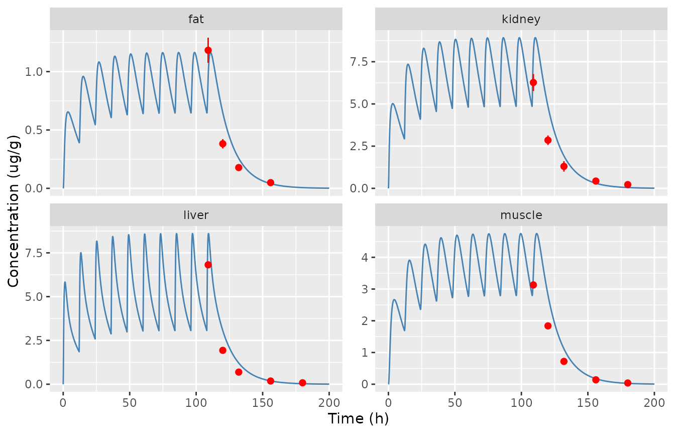
Replicates Figure 1 of Zhou 2021: enrofloxacin in muscle, fat, liver and kidney of a 55 kg pig after 5 mg/kg twice daily for 5 days. Lines: model; points: Table S2 mean +/- SD.
plot_tissues("CIP")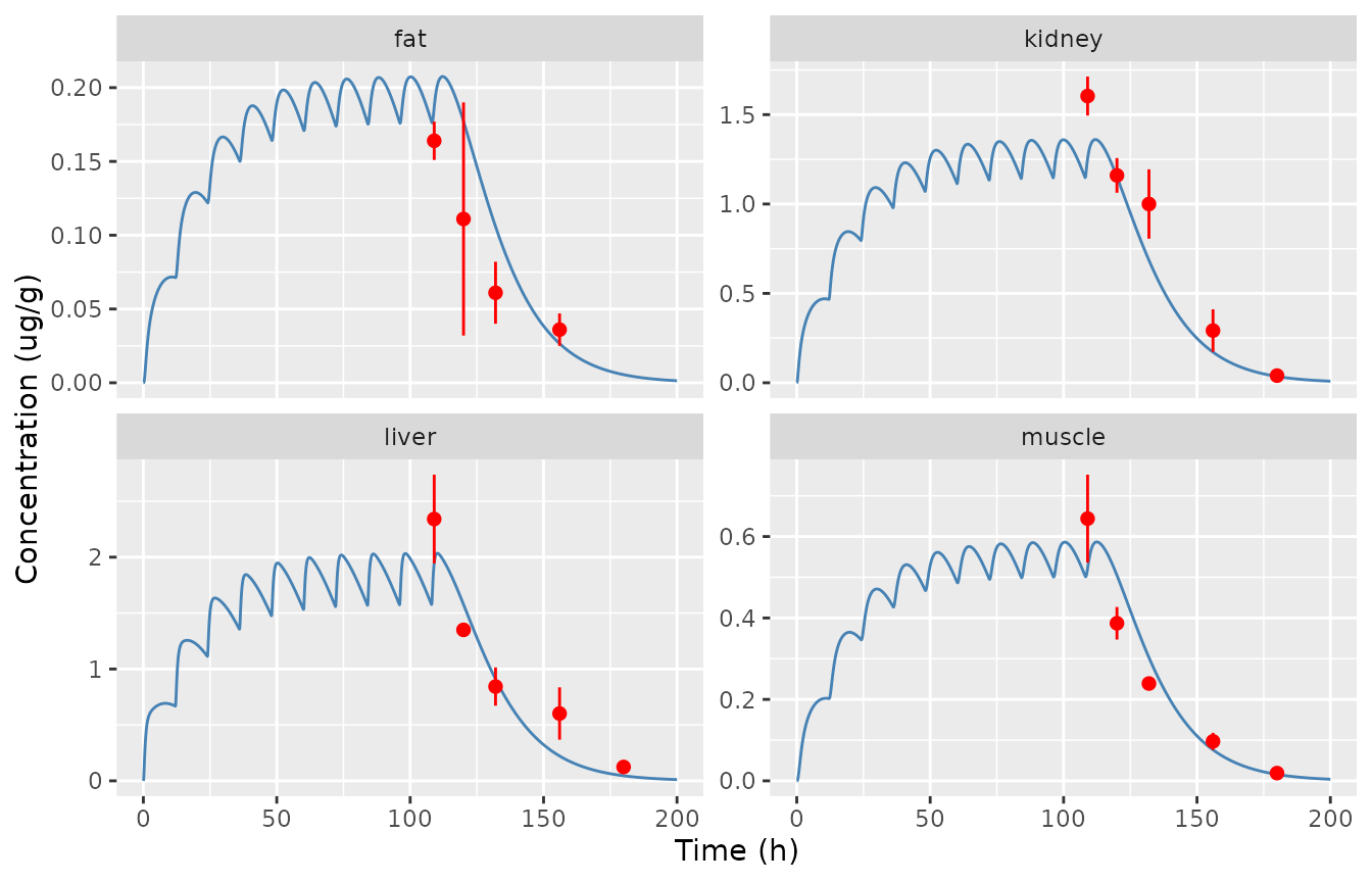
Replicates Figure 2 of Zhou 2021: ciprofloxacin in the four edible tissues.
plot_tissues("ENR + CIP")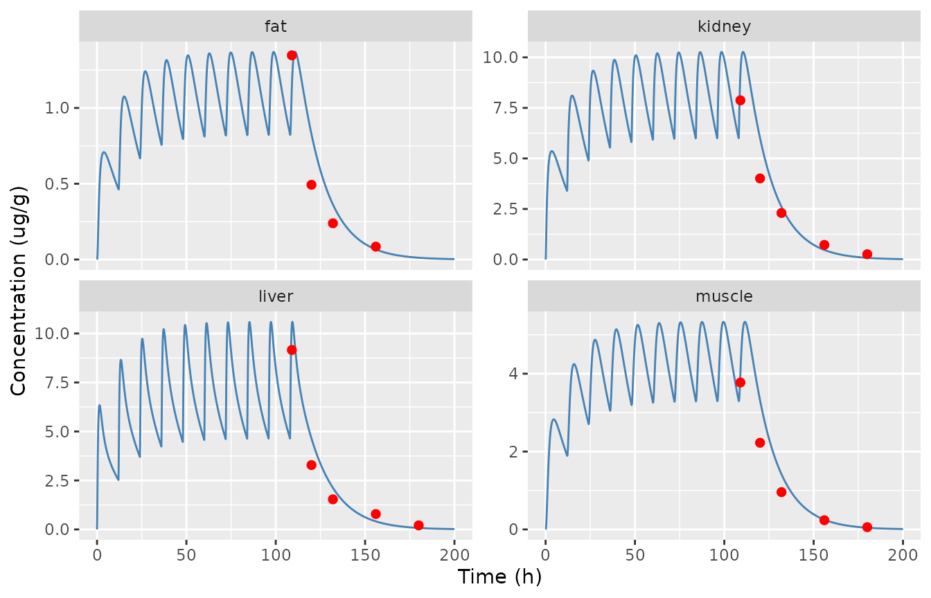
Replicates Figure 3 of Zhou 2021: the residue marker enrofloxacin + ciprofloxacin in the four edible tissues.
Zhou 2021 judged the calibration by linear regression of observed on predicted residue concentrations. Their acceptance criterion was R^2 >= 0.75 (Section 4.5), and they reported R^2 > 0.82 throughout (Figure S2). The same regression on the model predictions at the Table S2 sampling times:
pred_at_obs <- obs_long |>
  dplyr::mutate(time_key = round(time, 1)) |>
  dplyr::left_join(
    pred5 |> dplyr::mutate(time_key = round(time, 1)) |>
      dplyr::select(tissue, analyte, time_key, pred = conc),
    by = c("tissue", "analyte", "time_key")
  )
stopifnot(!anyNA(pred_at_obs$pred))
r2 <- pred_at_obs |>
  dplyr::group_by(analyte, tissue) |>
  dplyr::summarise(
    n = dplyr::n(),
    r2 = summary(stats::lm(conc ~ pred))$r.squared,
    median_ratio = stats::median(pred / conc),
    .groups = "drop"
  )
r2 |>
  dplyr::mutate(r2 = signif(r2, 3), median_ratio = signif(median_ratio, 3)) |>
  dplyr::rename(
    Analyte = analyte, Tissue = tissue, `Time points` = n, `R^2` = r2,
    `Median predicted / observed` = median_ratio
  ) |>
knitr::kable(caption = "Observed-vs-predicted regression per tissue and analyte (compare Zhou 2021 Figure S2).")| Analyte | Tissue | Time points | R^2 | Median predicted / observed |
|---|---|---|---|---|
| CIP | fat | 4 | 0.834 | 1.370 |
| CIP | kidney | 5 | 0.946 | 0.781 |
| CIP | liver | 5 | 0.896 | 0.832 |
| CIP | muscle | 5 | 0.866 | 0.832 |
| ENR | fat | 4 | 0.847 | 1.130 |
| ENR | kidney | 5 | 0.968 | 1.260 |
| ENR | liver | 5 | 0.992 | 1.250 |
| ENR | muscle | 5 | 0.955 | 1.260 |
| ENR + CIP | fat | 4 | 0.837 | 1.180 |
| ENR + CIP | kidney | 5 | 0.972 | 1.130 |
| ENR + CIP | liver | 5 | 0.985 | 1.140 |
| ENR + CIP | muscle | 5 | 0.946 | 1.060 |
# The paper's own acceptance criterion (Section 4.5). The comparison is
# deterministic (typical-value solve against fixed data), so it is exact.
stopifnot(all(r2$r2 >= 0.75))
The regression criterion passes in every tissue and analyte. The fit is not unbiased, though. Enrofloxacin is over-predicted (median predicted/observed about 1.1-1.3), most visibly at the 0.5-day and 1-day samples in muscle and liver, as in the paper’s own Figure 1. Ciprofloxacin is under-predicted by about 20% in muscle, liver and kidney. The two errors partly cancel in the enrofloxacin + ciprofloxacin residue marker, which is the quantity the withdrawal time is based on.
Liver-toxicity dose (Figure 5b)
Zhou 2021 took the in vitro IC50 of enrofloxacin against pig hepatocytes (225.9 ug/mL, Figure 5a) as a liver toxicity threshold. They report that 130 mg/kg twice daily for 5 days produces a liver enrofloxacin Cmax of 222.9 ug/mL at 109 h. The liver ciprofloxacin concentration at that time is 51.9 ug/mL (Section 2.4).
doses_tox <- c(30, 60, 130, 300, 600)
sim_tox <- dplyr::bind_rows(lapply(doses_tox, function(d) {
  rxode2::rxSolve(mod_typ, make_events(d, times = seq(0, 200, by = 0.1)), returnType = "data.frame") |>
    dplyr::mutate(dose = d)
}))
#> ℹ omega/sigma items treated as zero: 'etalkp_liver', 'etalkp_kidney', 'etalkp_muscle', 'etalkp_adipose', 'etalkp_liver_cipro', 'etalkp_kidney_cipro', 'etalkp_muscle_cipro', 'etalkp_adipose_cipro', 'etakmet', 'etafm', 'etalcl_renal', 'etalcl_renal_cipro'
#> ℹ omega/sigma items treated as zero: 'etalkp_liver', 'etalkp_kidney', 'etalkp_muscle', 'etalkp_adipose', 'etalkp_liver_cipro', 'etalkp_kidney_cipro', 'etalkp_muscle_cipro', 'etalkp_adipose_cipro', 'etakmet', 'etafm', 'etalcl_renal', 'etalcl_renal_cipro'
#> ℹ omega/sigma items treated as zero: 'etalkp_liver', 'etalkp_kidney', 'etalkp_muscle', 'etalkp_adipose', 'etalkp_liver_cipro', 'etalkp_kidney_cipro', 'etalkp_muscle_cipro', 'etalkp_adipose_cipro', 'etakmet', 'etafm', 'etalcl_renal', 'etalcl_renal_cipro'
#> ℹ omega/sigma items treated as zero: 'etalkp_liver', 'etalkp_kidney', 'etalkp_muscle', 'etalkp_adipose', 'etalkp_liver_cipro', 'etalkp_kidney_cipro', 'etalkp_muscle_cipro', 'etalkp_adipose_cipro', 'etakmet', 'etafm', 'etalcl_renal', 'etalcl_renal_cipro'
#> ℹ omega/sigma items treated as zero: 'etalkp_liver', 'etalkp_kidney', 'etalkp_muscle', 'etalkp_adipose', 'etalkp_liver_cipro', 'etalkp_kidney_cipro', 'etalkp_muscle_cipro', 'etalkp_adipose_cipro', 'etakmet', 'etafm', 'etalcl_renal', 'etalcl_renal_cipro'
fig5 <- dplyr::bind_rows(
  sim_tox |> dplyr::transmute(time, conc = Cliver, curve = paste0("ENR-", dose, " mg/kg")),
  sim_tox |> dplyr::filter(dose == 130) |>
    dplyr::transmute(time, conc = Cliver_cipro, curve = "CIP-130 mg/kg")
)
ggplot(fig5, aes(time, conc, colour = curve)) +
  geom_line() +
  geom_hline(yintercept = 225.9, linetype = "dashed") +
  labs(x = "Time (h)", y = "Liver concentration (ug/mL)", colour = NULL)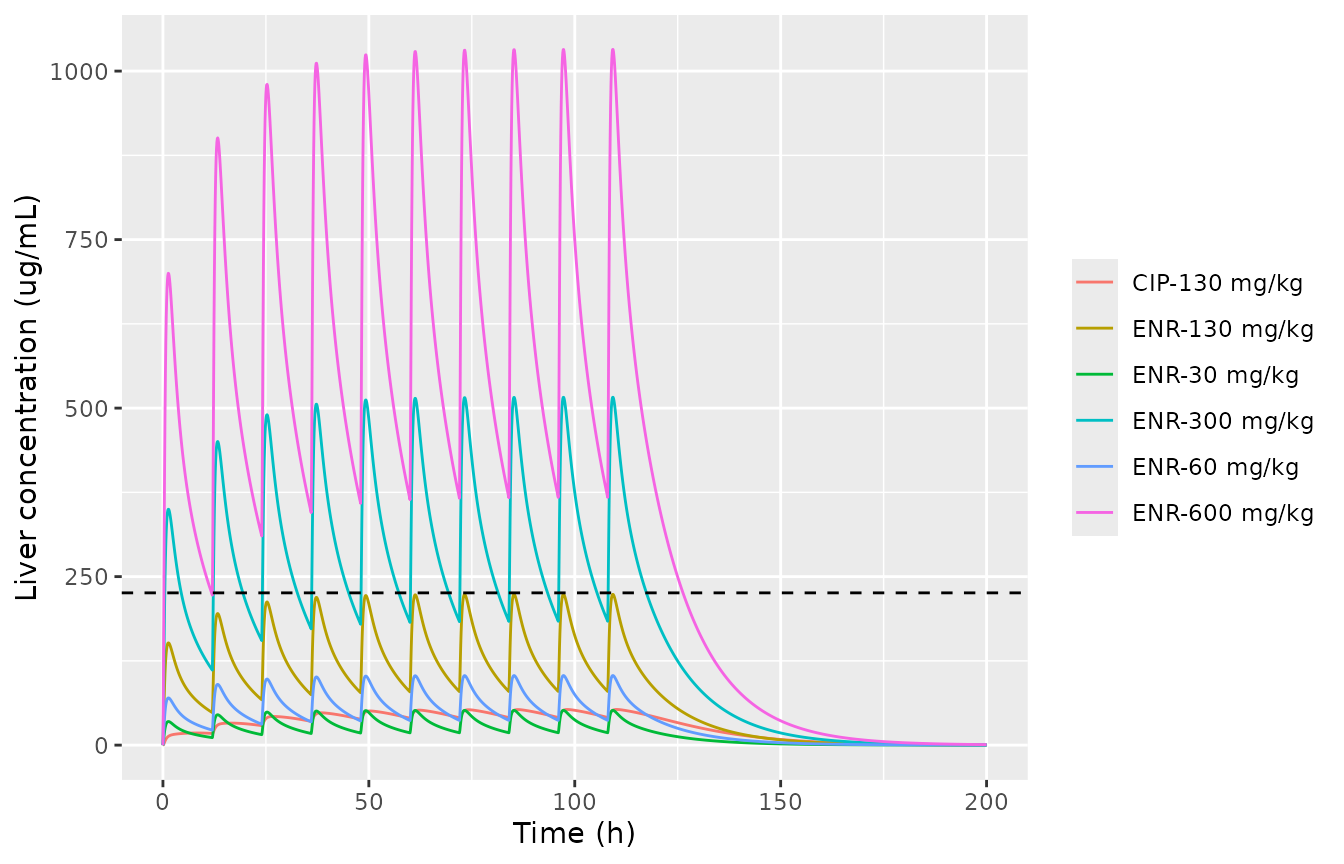
Replicates Figure 5b of Zhou 2021: liver enrofloxacin for 30-600 mg/kg twice daily for 5 days, and liver ciprofloxacin at 130 mg/kg. Dashed line: hepatocyte IC50 225.9 ug/mL.
last130 <- sim_tox |> dplyr::filter(dose == 130, time >= t_last, time <= t_last + 12)
i_max <- which.max(last130$Cliver)
tox_check <- data.frame(
  quantity = c("Liver ENR Cmax (ug/mL)", "Time of Cmax (h)", "Liver CIP at that time (ug/mL)"),
  published = c(222.9, 109, 51.9),
  model = c(last130$Cliver[i_max], last130$time[i_max], last130$Cliver_cipro[i_max])
)
tox_check$pct_diff <- 100 * (tox_check$model - tox_check$published) / tox_check$published
tox_check |>
  dplyr::mutate(model = signif(model, 4), pct_diff = round(pct_diff, 2)) |>
  dplyr::rename(Quantity = quantity, Published = published, Model = model, `% diff` = pct_diff) |>
knitr::kable(caption = "Zhou 2021 Section 2.4 values at 130 mg/kg against the model.")| Quantity | Published | Model | % diff |
|---|---|---|---|
| Liver ENR Cmax (ug/mL) | 222.9 | 223.60 | 0.33 |
| Time of Cmax (h) | 109.0 | 109.30 | 0.28 |
| Liver CIP at that time (ug/mL) | 51.9 | 51.88 | -0.04 |
# Deterministic typical-value solve against numbers the authors computed with
# the same equations, so the agreement is tight. The residual 0.3% on Cmax
# comes from the 0.001-h dosing pulse and the 0.1-h output interval of the
# acslX run.
stopifnot(
  abs(tox_check$pct_diff[1]) < 1,
  abs(tox_check$model[2] - 109) <= 0.5,
  abs(tox_check$pct_diff[3]) < 1
)

# The model is linear in dose, so the dose that brings the liver Cmax to the
# IC50 follows directly.
dose_ic50 <- 130 * 225.9 / last130$Cliver[i_max]
The model reproduces the three published numbers to within 0.4%. The liver ciprofloxacin value is the check that decides how File S2 converts ciprofloxacin to mass units; see the Errata. Because the model is linear in dose, the liver Cmax reaches the hepatocyte IC50 at 131.3 mg/kg. That matches the paper’s safe range of <= 130 mg/kg.
Mass balance
File S2 carries two mass-balance identities. For enrofloxacin, the
absorbed amount equals the amount in the body plus the amount excreted
in urine plus the amount metabolised (Bal = AAO - Tmass).
For ciprofloxacin, the formed amount (Frac * Amet) equals
the ciprofloxacin in the body plus that excreted in urine
(Bal1 = Amet1 - Tmass1). Adding the gut contents and faecal
loss closes the balance against the administered dose.
dose_umol <- 10 * 5 * wt_ref * 2.78
mb <- sim5 |>
  dplyr::mutate(
    tmass = venous + arterial + lung + liver + kidney + muscle + adipose + other +
      urine + a_metabolized,
    bal = a_oral_absorbed - tmass,
    tmass1 = venous_cipro + arterial_cipro + lung_cipro + liver_cipro + kidney_cipro +
      muscle_cipro + adipose_cipro + other_cipro + urine_cipro,
    bal1 = 0.35 * a_metabolized - tmass1
  )
mb_final <- mb[nrow(mb), ]
mb_final$bal_dose <- with(mb_final, stomach + intestine + a_feces + a_oral_absorbed - dose_umol)
data.frame(
  check = c("Bal / dose", "Bal1 / dose", "(gut + faeces + absorbed - dose) / dose"),
  value = signif(c(max(abs(mb$bal)), max(abs(mb$bal1)), abs(mb_final$bal_dose)) / dose_umol, 3)
) |>
  dplyr::rename(Check = check, `Max relative error` = value) |>
knitr::kable(caption = "Mass-balance identities of File S2 over 0-228 h.")| Check | Max relative error |
|---|---|
| Bal / dose | 0 |
| Bal1 / dose | 0 |
| (gut + faeces + absorbed - dose) / dose | 0 |
# Linear ODE with exact conservation; any error is solver round-off.
stopifnot(
  max(abs(mb$bal)) / dose_umol < 1e-6,
  max(abs(mb$bal1)) / dose_umol < 1e-6,
  abs(mb_final$bal_dose) / dose_umol < 1e-6
)
fate <- with(mb_final, c(
  urine_enrofloxacin = urine, metabolised = a_metabolized, faeces = a_feces
)) / dose_umol
knitr::kable(
  data.frame(Route = names(fate), `Fraction of dose at 228 h` = unname(signif(fate, 3)), check.names = FALSE),
  row.names = FALSE,
  caption = "Fate of the administered enrofloxacin at the end of the File S2 run (228 h)."
)| Route | Fraction of dose at 228 h |
|---|---|
| urine_enrofloxacin | 0.3730 |
| metabolised | 0.6090 |
| faeces | 0.0179 |
PKNCA
Zhou 2021 reports no conventional NCA table. The published liver Cmax and time of Cmax at 130 mg/kg (Section 2.4) are compared below with PKNCA run over the last dosing interval (108-120 h), with tmax relative to the last dose. Plasma NCA over the first dosing interval is included for reference.
liver_conc <- sim_tox |>
  dplyr::filter(time >= t_last, time <= t_last + 12, !is.na(Cliver)) |>
  dplyr::mutate(treatment = paste(dose, "mg/kg"), id = 1L, time = time - t_last) |>
  dplyr::select(id, treatment, time, Cliver)
liver_dose <- data.frame(id = 1L, treatment = paste(doses_tox, "mg/kg"), time = 0, amt = doses_tox * wt_ref)
nca_liver <- PKNCA::pk.nca(PKNCA::PKNCAdata(
  PKNCA::PKNCAconc(liver_conc, Cliver ~ time | treatment + id),
  PKNCA::PKNCAdose(liver_dose, amt ~ time | treatment + id),
  intervals = data.frame(start = 0, end = 12, cmax = TRUE, tmax = TRUE, auclast = TRUE)
))
published_nca <- data.frame(treatment = "130 mg/kg", cmax = 222.9, tmax = 1)
cmp <- nlmixr2lib::ncaComparisonTable(
  simulated = nca_liver,
  reference = published_nca,
  by = "treatment",
  params = c("cmax", "tmax"),
  units = c(cmax = "ug/mL", tmax = "h"),
  tolerance_pct = 20
)
knitr::kable(cmp, caption = "Liver enrofloxacin, last dosing interval: model (PKNCA) vs Zhou 2021 Section 2.4. * differs from the reference by more than 20%.")| NCA parameter | treatment | Reference | Simulated | % diff |
|---|---|---|---|---|
| Cmax (ug/mL) | 130 mg/kg | 223 | 224 | +0.3% |
| Tmax (h) | 130 mg/kg | 1 | 1.3 | +30.0%* |
plasma_conc <- sim5 |>
  dplyr::filter(time <= 12, !is.na(Cc)) |>
  dplyr::mutate(treatment = "5 mg/kg", id = 1L) |>
  dplyr::select(id, treatment, time, Cc)
plasma_dose <- data.frame(id = 1L, treatment = "5 mg/kg", time = 0, amt = 5 * wt_ref)
nca_plasma <- PKNCA::pk.nca(PKNCA::PKNCAdata(
  PKNCA::PKNCAconc(plasma_conc, Cc ~ time | treatment + id),
  PKNCA::PKNCAdose(plasma_dose, amt ~ time | treatment + id),
  intervals = data.frame(start = 0, end = 12, cmax = TRUE, tmax = TRUE, auclast = TRUE)
))
as.data.frame(nca_plasma) |>
  dplyr::select(treatment, PPTESTCD, PPORRES) |>
  dplyr::mutate(PPORRES = signif(PPORRES, 3)) |>
  dplyr::rename(Treatment = treatment, Parameter = PPTESTCD, Value = PPORRES) |>
knitr::kable(caption = "Plasma enrofloxacin, first dose (0-12 h), typical 55 kg pig. No published counterpart.")| Treatment | Parameter | Value |
|---|---|---|
| 5 mg/kg | auclast | 10.4 |
| 5 mg/kg | cmax | 1.1 |
| 5 mg/kg | tmax | 3.2 |
The liver Cmax agrees to 0.3%. The starred tmax row is not a real discrepancy: the paper states the time of Cmax as 109 h, i.e. 1 h after the last dose, to the nearest hour, while the model peaks at 109.3 h (1.3 h). On a 1-h reference, 0.3 h of rounding is 30%.
Monte Carlo withdrawal time
The population withdrawal time analysis (Section 4.7) sampled BW and 12 chemical-specific parameters from normal distributions. Each distribution used the Table S4 mean and SD and was bounded to mean +/- SD. The withdrawal time of a tissue is the first day after the last dose on which 99% of the virtual pigs are below the maximum residue limit for enrofloxacin + ciprofloxacin. The paper used 1000 virtual pigs; 200 are used here. The etas are drawn in R from the truncated normals and passed to the typical-value model as data columns, which override the zeroed etas.
set.seed(20210808)
n_mc <- 200
om <- rxode2::rxode2(mod)$omega
stopifnot(all(om[upper.tri(om)] == 0))
r_trunc <- function(n, sd) stats::qnorm(stats::runif(n, stats::pnorm(-1), stats::pnorm(1))) * sd
eta_draw <- as.data.frame(lapply(sqrt(diag(om)), function(s) r_trunc(n_mc, s)))
eta_draw$id <- seq_len(n_mc)
eta_draw$WT <- 55 + r_trunc(n_mc, 10)

t_wd <- t_last + 24 * (1:6)
ev_mc <- rxode2::et(amt = 1, cmt = "stomach", ii = 12, addl = 9) |>
  rxode2::et(c(0, t_wd), cmt = "venous") |>
  as.data.frame() |>
  dplyr::select(-dplyr::any_of("id")) |>
  dplyr::cross_join(eta_draw) |>
  dplyr::arrange(id, time, dplyr::desc(evid)) |>
  dplyr::mutate(amt = ifelse(evid == 1, 5 * WT, NA_real_))
sim_mc <- rxode2::rxSolve(mod_typ, ev_mc, returnType = "data.frame")
#> ℹ omega/sigma items treated as zero: 'etalkp_liver', 'etalkp_kidney', 'etalkp_muscle', 'etalkp_adipose', 'etalkp_liver_cipro', 'etalkp_kidney_cipro', 'etalkp_muscle_cipro', 'etalkp_adipose_cipro', 'etakmet', 'etafm', 'etalcl_renal', 'etalcl_renal_cipro'
#> Warning: multi-subject simulation without without 'omega'
stopifnot(!anyNA(sim_mc$Cliver_total), all(sim_mc$Cliver_total >= 0))

mrl <- c(muscle = 0.1, fat = 0.1, liver = 0.2, kidney = 0.3)
mc_cols <- c(muscle = "Cmuscle_total", fat = "Cadipose_total", liver = "Cliver_total", kidney = "Ckidney_total")
below <- dplyr::bind_rows(lapply(names(mrl), function(tis) {
  sim_mc |>
    dplyr::filter(time %in% t_wd) |>
    dplyr::group_by(time) |>
    dplyr::summarise(frac_below = mean(.data[[mc_cols[[tis]]]] < mrl[[tis]]), .groups = "drop") |>
    dplyr::mutate(tissue = tis, day = (time - t_last) / 24)
}))
# Zhou 2021 Figure 4: number of the 1000 virtual pigs below the MRL on each day.
fig4 <- tibble::tribble(
  ~tissue,  ~day, ~published_per_1000,
  "muscle", 2,    206,
  "muscle", 3,    833,
  "muscle", 4,    971,
  "muscle", 5,    991,
  "fat",    2,    993,
  "fat",    3,    990,
  "liver",  2,    306,
  "liver",  3,    905,
  "liver",  4,    968,
  "liver",  5,    988,
  "kidney", 2,    579,
  "kidney", 3,    976,
  "kidney", 4,    991
)
below |>
  dplyr::filter(day <= 5) |>
  dplyr::mutate(model_per_1000 = round(1000 * frac_below)) |>
  dplyr::left_join(fig4, by = c("tissue", "day")) |>
  dplyr::select(tissue, day, model_per_1000, published_per_1000) |>
  dplyr::rename(
    Tissue = tissue, `Day after last dose` = day,
    `Model (per 1000)` = model_per_1000, `Figure 4 (per 1000)` = published_per_1000
  ) |>
knitr::kable(caption = "Virtual pigs below the MRL (enrofloxacin + ciprofloxacin), per 1000.")| Tissue | Day after last dose | Model (per 1000) | Figure 4 (per 1000) |
|---|---|---|---|
| muscle | 1 | 0 | NA |
| muscle | 2 | 10 | 206 |
| muscle | 3 | 885 | 833 |
| muscle | 4 | 1000 | 971 |
| muscle | 5 | 1000 | 991 |
| fat | 1 | 0 | NA |
| fat | 2 | 840 | 993 |
| fat | 3 | 1000 | 990 |
| fat | 4 | 1000 | NA |
| fat | 5 | 1000 | NA |
| liver | 1 | 0 | NA |
| liver | 2 | 10 | 306 |
| liver | 3 | 945 | 905 |
| liver | 4 | 1000 | 968 |
| liver | 5 | 1000 | 988 |
| kidney | 1 | 0 | NA |
| kidney | 2 | 100 | 579 |
| kidney | 3 | 985 | 976 |
| kidney | 4 | 1000 | 991 |
| kidney | 5 | 1000 | NA |
wd <- below |>
  dplyr::group_by(tissue) |>
  dplyr::summarise(model_wt = min(day[frac_below >= 0.99]), .groups = "drop") |>
  dplyr::left_join(
    tibble::tribble(
      ~tissue,  ~predicted_paper, ~measured_paper,
      "muscle", 5, 3,
      "fat",    3, 2,
      "liver",  6, 4,
      "kidney", 4, 6
    ),
    by = "tissue"
  )
wd |>
  dplyr::rename(
    Tissue = tissue, `Model WT (d)` = model_wt,
    `Zhou 2021 PBPK WT (d)` = predicted_paper, `Measured WT, EMA WT1.4 (d)` = measured_paper
  ) |>
knitr::kable(caption = "Withdrawal times (compare Zhou 2021 Table S5).")| Tissue | Model WT (d) | Zhou 2021 PBPK WT (d) | Measured WT, EMA WT1.4 (d) |
|---|---|---|---|
| fat | 3 | 3 | 2 |
| kidney | 4 | 4 | 6 |
| liver | 4 | 6 | 4 |
| muscle | 4 | 5 | 3 |
The typical-value model reproduces the deterministic results above exactly. The Monte Carlo withdrawal times do not match. With the distributions as the Methods and Table S4 describe them, the virtual population is much narrower than the paper’s Figure 4. The paper has about 20% of pigs below the muscle MRL on day 2 and 58% below the kidney MRL on day 2. The typical pig is well above both limits on day 2 (muscle 0.25 against 0.1 ug/g, kidney 0.47 against 0.3 ug/g), so the paper’s spread cannot come from normals bounded at +/- 1 SD. The same parameters without the bound (plain normals) give negative partition coefficients or rate constants in some draws, which is presumably why the bound was set. The exact sampling the acslXtreme Monte Carlo module used is not recoverable from the paper. Figure 4 is also internally inconsistent for fat: its bar labels read 993 of 1000 pigs below the MRL on day 2 and 990 on day 3 (a count should not fall), yet Table S5 gives a fat withdrawal time of 3 d, which requires fewer than 990 on day 2. The model’s population layer should therefore be read as “the distributions as documented”, not as a reproduction of Figure 4.
Assumptions and deviations
-
Ciprofloxacin mass conversion. File S2 converts
ciprofloxacin amounts to mg with a constant
MW1mgthat is never assigned. The model usesMW1mg = MW1 / 1000 = 0.33134mg/umol, from theMW1 = 331.34g/mol the code declares. That reading reproduces the paper’s 51.9 ug/mL liver ciprofloxacin at the 130 mg/kg Cmax to 0.05%. Using the enrofloxacin factor 0.36 would give 56.4 ug/mL instead. -
Ciprofloxacin lung partition coefficient. File S2
declares
PLu1 = 4.3(also in Table S8) but its ciprofloxacin lung equation uses the enrofloxacinPLu(CVLu1 = CLu1/PLu). The equation is followed, so the model carries onlylkp_lung. The two values are equal, so predictions are unaffected unless a user changes the lung partition coefficient. -
Dosing. File S2 delivers each dose to the stomach
as a 0.001-h pulse; the model uses a bolus into
stomach. The oral dose is given in mg and converted to umol byf(stomach) = 2.78(File S2MWmol), because the code integrates amounts in umol. -
Unused routes. File S2 also codes intravenous,
intramuscular and subcutaneous inputs. All their doses are zero in this
study and the IM and SC absorption rate constants are 0 (Table S8), so
they are not carried. An intravenous dose in File S2 enters venous
blood; dose
venous(withf(stomach)not applying, so give the amount in umol) to reproduce it. -
Table S4 inconsistencies. The SD column is followed
for every eta. The Kurinec row prints a mean of 0.2 against the 0.12 of
Table S8 and File S2. Its SD of 0.036 is exactly 30% of 0.12, so 0.12 is
kept as the typical value. Its bounds (0.184-0.236) fit neither mean.
The Pl upper bound is printed 3.64, where mean + SD is 3.84. The Pm1 row
prints CV 0.2 but SD 0.5 with bounds 1.0-2.0, so the SD corresponds to a
33% CV. Section 4.7 lists a
Kintamong the sampled parameters, but no such parameter exists in the model or in Table S4. The BW CV is printed as 0.182 (i.e. 10/55). -
Monte Carlo etas. The etas are the Table S4 SDs
squared, additive on the linear scale, and their names follow the
package convention (
etalkp_liverforlkp_liver) even though they are not on the log scale. The +/- 1 SD truncation cannot be expressed in an eta. A plainrxSolve(mod, ...)therefore samples untruncated normals, which can give negative parameter values and non-finite concentrations in a small fraction of subjects. Draw truncated etas explicitly, as in the Monte Carlo section. -
No residual error. The paper reports no
residual-error model;
propSdis fixed to 0. -
Fixed versus adjusted parameters. Parameters taken
unchanged from Lin et al. 2016 (Kst, Kfeces, KmC, Frac, PB, PB1,
KurineC) are wrapped in
fixed(). The quantities Section 4.5 says were adjusted by hand to the residue data (Ka, Kurine1C and the partition coefficients) are not. None has a reported standard error. - Plasma (Figure S1). The plasma comparison in Figure S1 uses data from an earlier study by the same group (ref. 3) whose dose is not stated in the paper, so it is not reproduced here.
- Printing errors in the source. Table S2 prints the kidney ciprofloxacin SD at 0.042 d as “0.0.109” (read as 0.109). The Figure 5 caption gives the log IC50 in “mg/kg b.w.” where Figure 5a and the text use ug/mL. The File S2 header says the parameter values are in “Supplementary Tables 2 and 3”; they are in Tables S7 and S8.
- Literature check. No erratum or correction for this article was found on Europe PMC (checked 2026-09-28).