Infliximab (Samuels 2025)
Source:vignettes/articles/Samuels_2025_infliximab.Rmd
Samuels_2025_infliximab.RmdModel and source
- Citation: Samuels A, Irie K, Mizuno T, Reifenberg J, Punt N, Vinks AA, Minar P. Integrating early response biomarkers in pharmacokinetic models: A novel method to individualize the initial infliximab dose in patients with Crohn’s disease. Clin Transl Sci. 2025;18(2):e70086. doi:10.1111/cts.70086. Structural model and parameter values from: Xiong Y, Mizuno T, Colman R, Hyams J, Noe JD, Boyle B, et al. Real-world infliximab pharmacokinetic study informs an electronic health record-embedded dashboard to guide precision dosing in children with Crohn’s disease. Clin Pharmacol Ther. 2021;109(6):1639-1647. doi:10.1002/cpt.2148.
- Description: Two-compartment population PK model of intravenous infliximab in children and young adults with Crohn’s disease, extended with dose-number-driven trajectories of the four clearance biomarkers to forecast exposure during induction and early maintenance (Samuels 2025). The structural model, covariate exponents and variability are the Xiong 2021 real-world paediatric model (REFINE cohort), all held at the Xiong estimates: clearance scales with body weight, serum albumin, erythrocyte sedimentation rate (ESR), neutrophil CD64 activity ratio and antibody-to-infliximab concentration; V1 with weight; Q and V2 with weight at exponents 1 and 0.586. Samuels 2025 adds an Emax-in-dose-number function that predicts each biomarker from its pre-treatment value as baseline * exp(Emax * (n - 1) / (D50 - 1 + n - 1)) at infusion n, with D50 held at 1.1 and Emax estimated for weight (+0.046), albumin (+0.110), ESR (-0.978) and nCD64 (-0.362), so that the model anticipates the improvement in clearance biomarkers that accompanies a response to induction. Holding the infusion counter at 1 throughout reproduces the baseline-covariates-only Xiong prediction. Inter-individual variability on clearance only; residual error additive on log-transformed concentrations.
- Article: https://doi.org/10.1111/cts.70086 (open access; Data S1 holds Table S1 and the NONMEM code used for the predictions)
- Structural model: Xiong 2021, https://doi.org/10.1002/cpt.2148
mod <- rxode2::rxode(readModelDb("Samuels_2025_infliximab"))
#> ℹ parameter labels from comments will be replaced by 'label()'
Samuels 2025 asks a dosing question. Infliximab clearance in children with Crohn’s disease depends on body weight, serum albumin, the erythrocyte sedimentation rate (ESR) and the neutrophil CD64 activity ratio (nCD64), and those biomarkers improve as the patient responds to induction. A dose chosen from pre-treatment values therefore over-predicts clearance for the rest of induction. The paper fits a log-scale Emax function of the infusion number to each biomarker and plugs the predicted values into the Xiong 2021 population PK model, whose parameters it holds at the published estimates.
Population
The biomarker trajectories were estimated on 239 children and young adults with Crohn’s disease starting infliximab in two US cohorts (Samuels 2025 Table 1). REFINE (n = 78) was a prospective multicentre observational study at four centres from 2014 to 2019. APPDASH (n = 161) was a retrospective cohort at Cincinnati Children’s Hospital Medical Center from 2019 to 2021. Mean age at the first infusion was 13.6 (SD 3.7) years and 92.1% were under 18; 40.6% were female and 86.6% White. The mean starting dose was 7.7 (SD 2.3) mg/kg, higher in APPDASH (8.2) than in REFINE (6.5). Mean biomarkers at the first infusion were: weight 48.3 kg, albumin 3.3 g/dL, ESR 26 mm/h and nCD64 7.2.
The PK parameters themselves are not re-estimated here. They come from Xiong 2021, which fitted 671 peak and trough concentrations from the 78 REFINE patients.
str(readModelDb("Samuels_2025_infliximab")()$population)
#> List of 12
#>  $ species       : chr "human"
#>  $ n_subjects    : int 239
#>  $ n_studies     : int 2
#>  $ age_range     : chr "2-22 years (APPDASH inclusion criterion; REFINE enrolled children and young adults under 22)"
#>  $ age_mean      : chr "13.6 (SD 3.7) years at the first infusion; 92.1% under 18 years"
#>  $ weight_mean   : chr "48.3 (SD 20.5) kg at the first infusion"
#>  $ sex_female_pct: num 40.6
#>  $ race_ethnicity: chr "86.6% White"
#>  $ disease_state : chr "Crohn's disease starting infliximab (anti-TNF naive in REFINE); Paris location L1:L2:L3 = 31:46:162, behaviour "| __truncated__
#>  $ dose_range    : chr "intravenous infliximab, mean starting dose 7.7 (SD 2.3) mg/kg (REFINE 6.5, APPDASH 8.2 mg/kg); induction at wee"| __truncated__
#>  $ regions       : chr "United States (Cincinnati Children's Hospital Medical Center, Nationwide Children's Hospital, Medical College o"| __truncated__
#>  $ notes         : chr "Two cohorts: REFINE (prospective multicentre, n = 78, 2014-2019) and APPDASH (retrospective single-centre, n = "| __truncated__
Source trace
Every value in ini() carries an in-file comment naming
its source. In summary:
| Element | Value | Source |
|---|---|---|
| CL (65 kg, ALB 3.5 g/dL, ESR 9 mm/h, nCD64 4.6) | 0.0138 L/h | Data S1 THETA(1); Xiong 2021 Table 2 |
| V1 (65 kg) | 2.97 L | Data S1 THETA(2); Xiong 2021 Table 2 |
| Q (65 kg) | 0.00953 L/h | Data S1 THETA(3); Xiong 2021 Table 2 (0.0095) |
| V2 (65 kg) | 2.84 L | Data S1 THETA(4); Xiong 2021 Table 2 |
| Albumin exponent on CL | -1.07 | Data S1 THETA(5); Xiong 2021 Table 2 |
| ATI exponent on CL (above 22 ng/mL) | 0.134 | Data S1 THETA(6) and IF(ATI.LE.22) branch; Xiong 2021
Table 2 |
| nCD64 exponent on CL | 0.168 | Data S1 THETA(7); Xiong 2021 Table 2 |
| ESR exponent on CL | 0.101 | Data S1 THETA(8); Xiong 2021 Table 2 |
| Weight exponent on CL | 0.594 | Data S1 THETA(9) ‘CLWT1’; Xiong 2021 Table 2 (see Assumptions) |
| Weight exponent on V1 | 0.55 | Data S1 THETA(10) ‘V1WT1’; Xiong 2021 Table 2 |
| Weight exponents on Q and V2 | 1 and 0.586 | Data S1 $PK code; Xiong 2021 Table 2 |
| Emax, weight | 0.046 | Table S1; Data S1 E2; Results; Figure 1a |
| Emax, albumin | 0.110 | Table S1; Data S1 E1; Results; Figure 1b |
| Emax, ESR | -0.978 | Table S1; Data S1 E3; Results; Figure 1c |
| Emax, nCD64 | -0.362 | Table S1; Data S1 E4; Results; Figure 1d |
| D50 | 1.1 (held) | Methods; Data S1 constant 0.1 = D50 - 1 |
| IIV on CL | 0.0629 | Data S1 OMEGA(1,1); Xiong 2021 Table 2 (25.1% CV) |
| IIV on V1, Q, V2 | 0 (omitted) | Data S1 OMEGA(2)-(4) |
| Residual SD, log scale | sqrt(0.189) = 0.4347 | Data S1 $SIGMA; Xiong 2021 Table 2 (0.435) |
| Trajectory equation | biomarker = E0 * exp(Emax * (n - 1) / (D50 - 1 + n - 1)) | Methods equation; Data S1 E1-E4 |
| CL equation | power product of the predicted biomarkers and thresholded ATI | Data S1 $PK; Xiong 2021 Table 2 footnote |
| Residual model | Y = log(F) + EPS | Data S1 $ERROR
|
Biomarker trajectories (Figure 1)
The Emax function predicts each biomarker from its pre-treatment
value at infusion number n. Because the D50 of 1.1 sits
just above the first infusion, nearly the whole change, 1 / 1.1 = 91% of
it, is in place by the second infusion.
theta <- rxode2::rxode(readModelDb("Samuels_2025_infliximab"))$theta
#> ℹ parameter labels from comments will be replaced by 'label()'
e0 <- c(
  "Weight (kg)" = 48.8, "Albumin (g/dL)" = 3.3,
  "ESR (mm/h)" = 27.6, "nCD64 (ratio)" = 7.7
)
emax <- c(
  "Weight (kg)" = theta[["wt_dosenum_max"]],
  "Albumin (g/dL)" = theta[["alb_dosenum_max"]],
  "ESR (mm/h)" = theta[["erythrocyte_sedimentation_rate_dosenum_max"]],
  "nCD64 (ratio)" = theta[["neutrophil_cd64_ratio_dosenum_max"]]
)
d50 <- theta[["dosenum50"]]
traj <- expand.grid(n = seq(1, 4, by = 0.01), biomarker = names(e0)) |>
  mutate(
    value = e0[as.character(biomarker)] *
      exp(emax[as.character(biomarker)] * (n - 1) / (d50 - 1 + n - 1))
  )
ggplot(traj, aes(n, value)) +
  geom_line() +
  facet_wrap(~biomarker, scales = "free_y") +
  expand_limits(y = 0) +
  labs(
    x = "Dose number", y = "Predicted biomarker",
    caption = "Replicates the fitted curves of Figure 1 of Samuels 2025 (E0 from Table S1)."
  )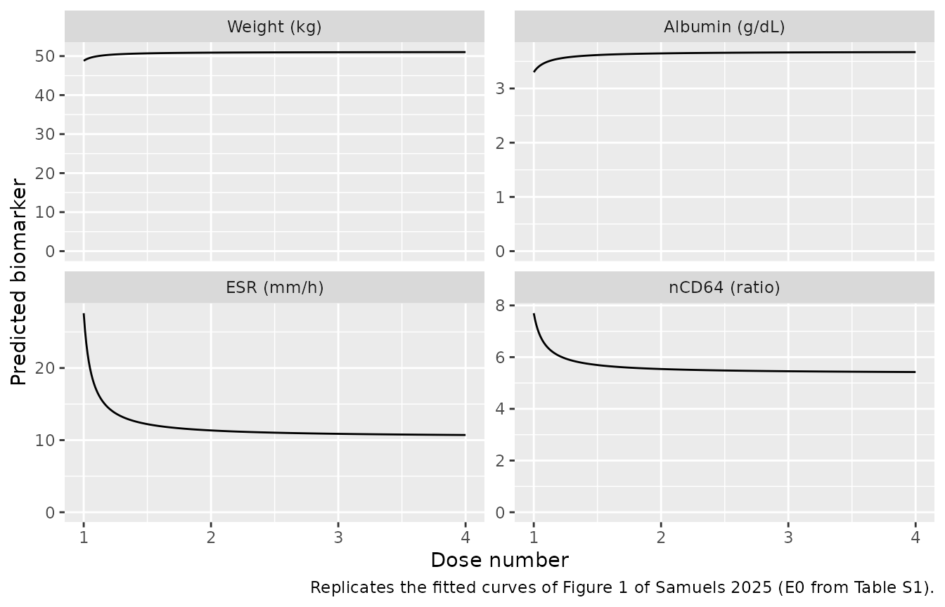
The Results quote each Emax as an asymptotic percentage change,
exp(Emax) - 1. Three of the four reproduce:
pct_chk <- data.frame(
  biomarker = names(emax),
  row.names = NULL,
  paper_pct = c(4.7, 11.7, -62.4, -26.5),
  model_pct = unname(round(100 * (exp(emax) - 1), 1))
)
knitr::kable(pct_chk |>
  dplyr::rename(
    Biomarker = biomarker,
    "Results / Figure 1 (%)" = paper_pct,
    "100 * (exp(Emax) - 1) (%)" = model_pct
))| Biomarker | Results / Figure 1 (%) | 100 * (exp(Emax) - 1) (%) |
|---|---|---|
| Weight (kg) | 4.7 | 4.7 |
| Albumin (g/dL) | 11.7 | 11.6 |
| ESR (mm/h) | -62.4 | -62.4 |
| nCD64 (ratio) | -26.5 | -30.4 |
The nCD64 Emax of -0.362 gives -30.4%, not the -26.5% printed in the Results and in the Figure 1d title. The value -0.362 is printed in three places (Table S1, the Data S1 code and the Figure 1d title), so it is the one encoded. The -26.5% matches neither the estimate nor the bootstrap median (-0.404), and is treated as a typographical error in the percentage.
Figure 2: a 47 kg patient on 5 or 10 mg/kg
Samuels 2025 Figure 2 simulates infusions at weeks 0, 2, 6 and 14 for a 47 kg patient, with and without the predicted biomarker improvement. The paper does not state the other pre-treatment biomarkers used, so the Table S1 E0 values (albumin 3.3 g/dL, ESR 27.6 mm/h, nCD64 7.7) are used here, with no antibodies to infliximab.
How the infusion counter is set
CYCLE is the 1-based infusion number, and the model
forms the paper’s zero-based INFUSION = CYCLE - 1. The Emax
equation defines a biomarker value at each infusion visit but not
between visits. Figure 2 shows the two curves separating before the
second infusion. That is the NONMEM convention in which a record’s
covariates govern the interval that ends at that record: the interval
after infusion k takes the biomarker values of visit
k + 1. In rxode2, which carries covariates forward, the
same thing is done by giving every record after infusion k
the value CYCLE = k + 1. For the baseline-only prediction,
CYCLE stays at 1 throughout.
dose_wk <- c(0, 2, 6, 14)
dose_h <- dose_wk * 7 * 24
inf_dur <- 2 # h; the paper does not state the infusion duration
obs_h <- sort(unique(c(seq(0, 22 * 168, by = 6), dose_h + inf_dur)))

make_events <- function(id, mgkg, scenario, wt = 47, alb_gdl = 3.3,
                        esr = 27.6, ncd64 = 7.7, ada = 0) {
  amt <- mgkg * wt
  dose <- data.frame(
    id = id, time = dose_h, amt = amt, rate = amt / inf_dur,
    evid = 1L, cmt = "central"
  )
  obs <- data.frame(
    id = id, time = obs_h, amt = 0, rate = 0, evid = 0L, cmt = "central"
  )
  ev <- dplyr::bind_rows(dose, obs) |>
    dplyr::arrange(time, dplyr::desc(evid))
  # Closing-visit convention: after infusion k, CYCLE = k + 1.
  ev$CYCLE <- if (scenario == "Time-varying biomarkers") {
    findInterval(ev$time, dose_h) + 1L
  } else {
    1L
  }
  ev$WT <- wt
  ev$ALB <- alb_gdl * 10 # g/dL -> canonical g/L
  ev$ERYTHROCYTE_SEDIMENTATION_RATE <- esr
  ev$NEUTROPHIL_CD64_RATIO <- ncd64
  ev$CONC_ADA_NGML <- ada
  ev$treatment <- paste0(mgkg, " mg/kg")
  ev$scenario <- scenario
  ev
}

scen <- c("Time-varying biomarkers", "Baseline biomarkers only")
ev_fig2 <- dplyr::bind_rows(
  make_events(1, 5, scen[1]), make_events(2, 5, scen[2]),
  make_events(3, 10, scen[1]), make_events(4, 10, scen[2])
)
sim_fig2 <- rxode2::rxSolve(
  rxode2::zeroRe(mod), ev_fig2,
  keep = c("treatment", "scenario"), returnType = "data.frame"
)
#> ℹ omega/sigma items treated as zero: 'etalcl'
#> Warning: multi-subject simulation without without 'omega'
ggplot(sim_fig2, aes(time / 168, Cc, linetype = scenario, colour = scenario)) +
  geom_line() +
  scale_y_log10(limits = c(1, NA)) +
  scale_x_continuous(breaks = seq(0, 22, by = 2)) +
  facet_wrap(~treatment, ncol = 1) +
  scale_colour_manual(values = c("black", "purple")) +
  labs(
    x = "Time (weeks)", y = "Infliximab (ug/mL)", colour = NULL, linetype = NULL,
    caption = "Replicates Figure 2 of Samuels 2025 (typical patient, no IIV)."
  ) +
  theme(legend.position = "bottom")
#> Warning in scale_y_log10(limits = c(1, NA)): log-10 transformation introduced
#> infinite values.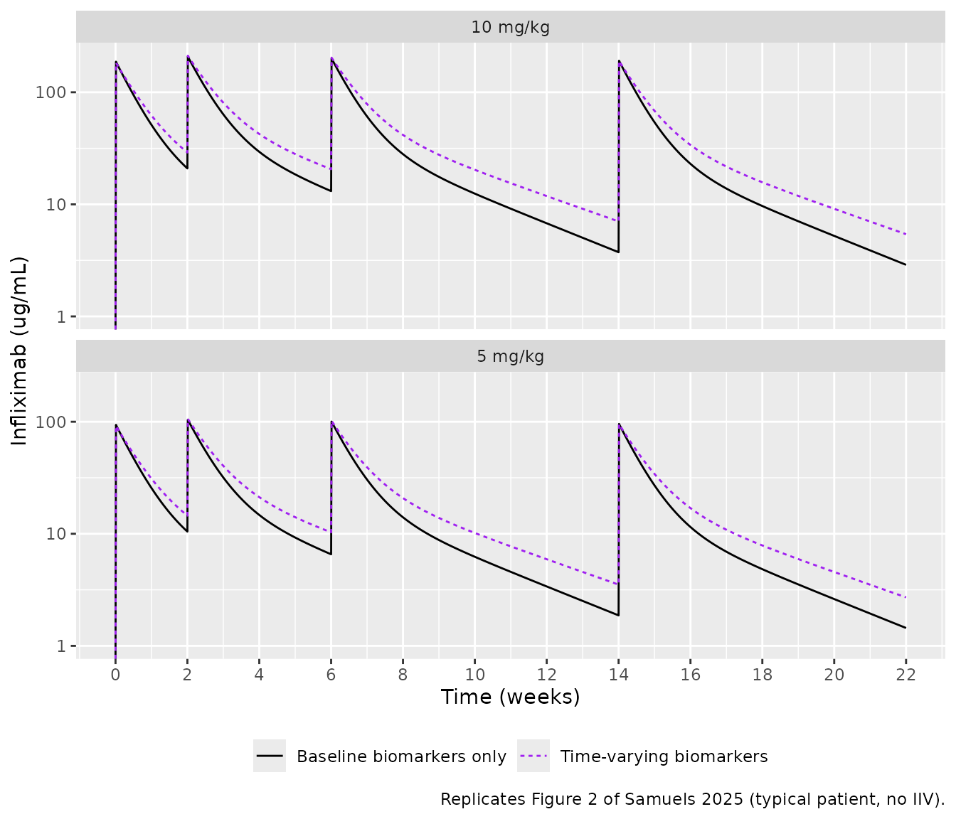
Troughs read from Figure 2a (5 mg/kg) by the maintainers, against the simulation:
trough_h <- c(2, 6, 14) * 168
fig2 <- data.frame(
  week = c(2, 6, 14),
  paper_tv = c(16.0, 12.8, 4.7),
  paper_base = c(12.8, 8.6, 2.6)
)
sim_tr <- sim_fig2 |>
  dplyr::filter(treatment == "5 mg/kg", time %in% trough_h) |>
  dplyr::mutate(week = time / 168) |>
  dplyr::select(week, scenario, Cc) |>
  tidyr::pivot_wider(names_from = scenario, values_from = Cc)
fig2_cmp <- fig2 |>
  dplyr::left_join(sim_tr, by = "week") |>
  dplyr::mutate(
    paper_ratio = paper_tv / paper_base,
    sim_ratio = `Time-varying biomarkers` / `Baseline biomarkers only`
  )
knitr::kable(
  fig2_cmp |>
    dplyr::rename(
      "Week (trough)" = week,
      "Figure 2a, time-varying" = paper_tv,
      "Figure 2a, baseline only" = paper_base,
      "Model, time-varying" = `Time-varying biomarkers`,
      "Model, baseline only" = `Baseline biomarkers only`,
      "Figure 2a ratio" = paper_ratio,
      "Model ratio" = sim_ratio
    ),
  digits = 2
)| Week (trough) | Figure 2a, time-varying | Figure 2a, baseline only | Model, time-varying | Model, baseline only | Figure 2a ratio | Model ratio |
|---|---|---|---|---|---|---|
| 2 | 16.0 | 12.8 | 14.52 | 10.46 | 1.25 | 1.39 |
| 6 | 12.8 | 8.6 | 10.30 | 6.56 | 1.49 | 1.57 |
| 14 | 4.7 | 2.6 | 3.52 | 1.87 | 1.81 | 1.88 |
The ratio of the two predictions is the quantity the paper is about. It depends on the Emax trajectories and the covariate exponents, not on the dose or on the unreported baseline biomarkers, and the model reproduces it closely. The week-2 ratio is the one most sensitive to how the counter is stepped within the first interval, which the paper does not describe.
Both absolute curves sit 10-30% below the figure. With linear PK and a ratio that agrees, the gap points to lower clearance in the paper’s typical patient, most likely from pre-treatment ESR and nCD64 values below the Table S1 means (for example cohort medians, which the paper does not report). Setting every biomarker to its reference value instead puts the baseline-only troughs above the figure (15.0, 10.7 and 3.7 ug/mL), so the figure’s patient lies between the two.
Virtual cohort and Table 3
Table 3 of Samuels 2025 compares observed troughs with population predictions from the baseline biomarkers (scenario a) and from the predicted trajectories (scenario b). The virtual cohort below draws pre-treatment biomarkers and starting doses from the Table 1 means and SDs. The doses and sampling of the real patients are not available, so the absolute medians are approximate. The ratio of scenario b to scenario a is the comparison that carries over.
set.seed(20250222)
n_sub <- 200
lnorm_draw <- function(n, m, s) {
  sdlog <- sqrt(log(1 + (s / m)^2))
  rlnorm(n, log(m) - sdlog^2 / 2, sdlog)
}
cohort <- data.frame(
  id = seq_len(n_sub),
  wt = pmin(pmax(lnorm_draw(n_sub, 48.3, 20.5), 15), 120),
  alb = pmin(pmax(rnorm(n_sub, 3.3, 0.61), 1.5), 5),
  esr = pmax(lnorm_draw(n_sub, 26, 24), 1),
  ncd64 = pmax(lnorm_draw(n_sub, 7.2, 4.6), 1),
  mgkg = round(pmin(pmax(rnorm(n_sub, 7.7, 2.3), 5), 10))
)

trough_events <- function(row, scenario, id) {
  amt <- row$mgkg * row$wt
  dose <- data.frame(
    id = id, time = dose_h, amt = amt, rate = amt / inf_dur,
    evid = 1L, cmt = "central"
  )
  obs <- data.frame(
    id = id, time = trough_h - 0.01, amt = 0, rate = 0,
    evid = 0L, cmt = "central"
  )
  ev <- dplyr::bind_rows(dose, obs) |>
    dplyr::arrange(time, dplyr::desc(evid))
  ev$CYCLE <- if (scenario == "b") findInterval(ev$time, dose_h) + 1L else 1L
  ev$WT <- row$wt
  ev$ALB <- row$alb * 10
  ev$ERYTHROCYTE_SEDIMENTATION_RATE <- row$esr
  ev$NEUTROPHIL_CD64_RATIO <- row$ncd64
  ev$CONC_ADA_NGML <- 0
  ev$scenario <- scenario
  ev
}
ev_cohort <- dplyr::bind_rows(lapply(seq_len(n_sub), function(i) {
  dplyr::bind_rows(
    trough_events(cohort[i, ], "a", i),
    trough_events(cohort[i, ], "b", n_sub + i)
  )
}))
sim_cohort <- rxode2::rxSolve(
  rxode2::zeroRe(mod), ev_cohort,
  keep = "scenario", returnType = "data.frame"
) |>
  dplyr::mutate(dose = c(2, 3, 4)[match(round(time), round(trough_h - 0.01))])
#> ℹ omega/sigma items treated as zero: 'etalcl'
#> Warning: multi-subject simulation without without 'omega'

tab3 <- data.frame(
  dose = c(2, 3, 4),
  observed = c(22, 19, 7.1),
  paper_a = c(12.8, 10.7, 4.9),
  paper_b = c(17.7, 16.9, 8.5)
)
sim_tab3 <- sim_cohort |>
  dplyr::group_by(dose, scenario) |>
  dplyr::summarise(median_cc = median(Cc), .groups = "drop") |>
  tidyr::pivot_wider(names_from = scenario, values_from = median_cc, names_prefix = "sim_")
sub_ratio <- sim_cohort |>
  dplyr::mutate(subj = ifelse(scenario == "b", id - n_sub, id)) |>
  dplyr::select(subj, dose, scenario, Cc) |>
  tidyr::pivot_wider(names_from = scenario, values_from = Cc) |>
  dplyr::group_by(dose) |>
  dplyr::summarise(sim_ratio = median(b / a))
tab3_cmp <- tab3 |>
  dplyr::left_join(sim_tab3, by = "dose") |>
  dplyr::left_join(sub_ratio, by = "dose") |>
  dplyr::mutate(paper_ratio = paper_b / paper_a)
knitr::kable(
  tab3_cmp |>
    dplyr::rename(
      "Trough before dose" = dose,
      "Observed median" = observed,
      "Table 3, scenario a" = paper_a,
      "Table 3, scenario b" = paper_b,
      "Model median, a" = sim_a,
      "Model median, b" = sim_b,
      "Model median ratio b/a" = sim_ratio,
      "Table 3 ratio b/a" = paper_ratio
    ),
  digits = 2,
  caption = "Median trough concentrations (ug/mL), Samuels 2025 Table 3 against the virtual cohort."
)| Trough before dose | Observed median | Table 3, scenario a | Table 3, scenario b | Model median, a | Model median, b | Model median ratio b/a | Table 3 ratio b/a |
|---|---|---|---|---|---|---|---|
| 2 | 22.0 | 12.8 | 17.7 | 16.34 | 22.20 | 1.37 | 1.38 |
| 3 | 19.0 | 10.7 | 16.9 | 10.05 | 15.84 | 1.56 | 1.58 |
| 4 | 7.1 | 4.9 | 8.5 | 3.03 | 5.63 | 1.85 | 1.73 |
The model’s ratio of scenario b to scenario a reproduces Table 3 closely before the second and third infusions (1.38 and 1.58 in the paper) and is about 7% higher before the fourth (1.73 in the paper). That comparison sets the median of per-patient ratios here against a ratio of medians over different patient subsets in the paper, so agreement within 10-15% is what can be expected. The absolute medians differ more, because the virtual cohort’s doses and covariates are drawn from Table 1 summaries rather than from the patients who contributed each trough.
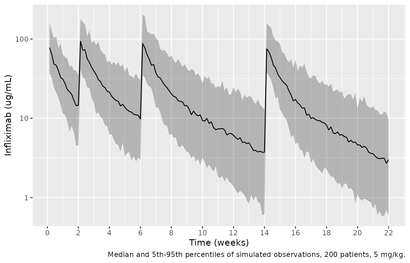
Stochastic simulation
With the IIV on clearance and the log-scale residual error, 200 virtual patients on 5 mg/kg with the time-varying biomarkers:
rxode2::rxSetSeed(20250222)
ev_vpc <- dplyr::bind_rows(lapply(seq_len(n_sub), function(i) {
  ev <- make_events(i, 5, scen[1],
    wt = cohort$wt[i], alb_gdl = cohort$alb[i],
    esr = cohort$esr[i], ncd64 = cohort$ncd64[i]
  )
  ev[ev$evid == 1L | (ev$time %% 24 == 0 & ev$time >= 24), ]
}))
sim_vpc <- rxode2::rxSolve(mod, ev_vpc, returnType = "data.frame")
vpc_sum <- sim_vpc |>
  dplyr::group_by(time) |>
  dplyr::summarise(
    p05 = quantile(sim, 0.05), p50 = quantile(sim, 0.5), p95 = quantile(sim, 0.95)
  )
ggplot(vpc_sum, aes(time / 168)) +
  geom_ribbon(aes(ymin = p05, ymax = p95), alpha = 0.3) +
  geom_line(aes(y = p50)) +
  scale_y_log10() +
  scale_x_continuous(breaks = seq(0, 22, by = 2)) +
  labs(
    x = "Time (weeks)", y = "Infliximab (ug/mL)",
    caption = "Median and 5th-95th percentiles of simulated observations, 200 patients, 5 mg/kg."
  )
PKNCA
Non-compartmental analysis per dosing interval of the Figure 2 typical-patient simulations. Intervals 2 to 4 close on the week 6, 14 and 22 troughs.
conc <- sim_fig2 |>
  dplyr::filter(!is.na(Cc)) |>
  dplyr::mutate(id = paste(treatment, scenario)) |>
  dplyr::select(id, time, Cc, treatment, scenario)
doses <- ev_fig2 |>
  dplyr::filter(evid == 1L) |>
  dplyr::mutate(id = paste(treatment, scenario)) |>
  dplyr::select(id, time, amt, treatment, scenario)
o_conc <- PKNCA::PKNCAconc(conc, Cc ~ time | treatment + scenario + id)
o_dose <- PKNCA::PKNCAdose(doses, amt ~ time | treatment + scenario + id)
intervals <- data.frame(
  start = dose_h,
  end = c(dose_h[-1], 22 * 168),
  cmax = TRUE, auclast = TRUE, cmin = c(FALSE, TRUE, TRUE, TRUE)
)
nca <- PKNCA::pk.nca(PKNCA::PKNCAdata(o_conc, o_dose, intervals = intervals))
nca_tbl <- as.data.frame(nca$result) |>
  dplyr::filter(PPTESTCD %in% c("cmax", "cmin", "auclast")) |>
  dplyr::mutate(interval = paste0("week ", start / 168, "-", end / 168)) |>
  dplyr::select(treatment, scenario, interval, PPTESTCD, PPORRES) |>
  tidyr::pivot_wider(names_from = PPTESTCD, values_from = PPORRES)
knitr::kable(
  nca_tbl |>
    dplyr::rename(
      Dose = treatment, Scenario = scenario, Interval = interval,
      "Cmax (ug/mL)" = cmax, "AUClast (ug*h/mL)" = auclast,
      "Cmin (ug/mL)" = cmin
    ),
  digits = 1
)| Dose | Scenario | Interval | AUClast (ug*h/mL) | Cmax (ug/mL) | Cmin (ug/mL) |
|---|---|---|---|---|---|
| 10 mg/kg | Baseline biomarkers only | week 0-2 | 22641.3 | 187.5 | NA |
| 10 mg/kg | Baseline biomarkers only | week 2-6 | 33536.7 | 208.3 | 13.1 |
| 10 mg/kg | Baseline biomarkers only | week 6-14 | 36964.1 | 200.6 | 3.7 |
| 10 mg/kg | Baseline biomarkers only | week 14-22 | 32236.6 | 191.2 | 2.9 |
| 10 mg/kg | Time-varying biomarkers | week 0-2 | 25456.9 | 183.5 | NA |
| 10 mg/kg | Time-varying biomarkers | week 2-6 | 41798.8 | 212.1 | 20.6 |
| 10 mg/kg | Time-varying biomarkers | week 6-14 | 48988.5 | 203.8 | 7.0 |
| 10 mg/kg | Time-varying biomarkers | week 14-22 | 41575.3 | 190.2 | 5.4 |
| 5 mg/kg | Baseline biomarkers only | week 0-2 | 11320.6 | 93.8 | NA |
| 5 mg/kg | Baseline biomarkers only | week 2-6 | 16768.3 | 104.1 | 6.6 |
| 5 mg/kg | Baseline biomarkers only | week 6-14 | 18482.1 | 100.3 | 1.9 |
| 5 mg/kg | Baseline biomarkers only | week 14-22 | 16118.3 | 95.6 | 1.4 |
| 5 mg/kg | Time-varying biomarkers | week 0-2 | 12728.5 | 91.7 | NA |
| 5 mg/kg | Time-varying biomarkers | week 2-6 | 20899.4 | 106.1 | 10.3 |
| 5 mg/kg | Time-varying biomarkers | week 6-14 | 24494.2 | 101.9 | 3.5 |
| 5 mg/kg | Time-varying biomarkers | week 14-22 | 20787.6 | 95.1 | 2.7 |
Samuels 2025 reports no NCA parameters, so the comparison against the paper is the Figure 2 and Table 3 trough comparison above. Two properties of the model are checked here. Because the PK is linear, the 10 mg/kg exposures are exactly twice the 5 mg/kg ones. And the first-interval Cmax is the same in both scenarios to within the small change in V1 that the predicted weight gain causes.
auc_ratio <- nca_tbl |>
  dplyr::select(treatment, scenario, interval, auclast) |>
  tidyr::pivot_wider(names_from = treatment, values_from = auclast) |>
  dplyr::mutate(r = `10 mg/kg` / `5 mg/kg`)
cmax1 <- nca_tbl |>
  dplyr::filter(interval == "week 0-2", treatment == "5 mg/kg")
stopifnot(
  all(abs(auc_ratio$r - 2) < 1e-3),
  abs(cmax1$cmax[1] / cmax1$cmax[2] - 1) < 0.05
)
Assumptions and deviations
-
Weight exponent on CL. The Data S1 code has a typo
in its THETA indices. Its non-missing-weight branch is
CLWT=((WT*E2)/65)**THETA(10), which would use the V1 weight exponent (0.55) on clearance. Its missing-weight branch for V1 citesTHETA(11), which the$THETAblock (ten entries) does not define. The$THETAlabels (THETA(9) ‘CLWT1’ = 0.594, THETA(10) ‘V1WT1’ = 0.55), the missing-weight branch for CL (E2**THETA(9)) and the Xiong 2021 final model (‘Weight for CL’ 0.594, ‘Weight for V1’ 0.55) all agree. The model therefore uses 0.594 on CL and 0.55 on V1. The difference is small: at 47 kg the CL weight factor is 0.825 with 0.594 and 0.837 with 0.55. -
Missing covariates. The Data S1 code handles a
missing biomarker (
-99) by applying only the trajectory factor, for exampleE1**THETA(5). That equals the full expression evaluated at the reference value, so a missing value should be imputed with the reference (65 kg, 3.5 g/dL, 9 mm/h, 4.6) rather than handled in the model. - Baseline weight on Q and V2. As in the Data S1 code, the predicted weight scales CL and V1, while Q and V2 are scaled by the pre-treatment weight.
-
Infusion counter between visits. The paper defines
the trajectories at infusion visits only. The vignette applies the visit
k + 1values over the interval after infusionk, which reproduces the shape of Figure 2 (see above). A user who prefers to apply visitkvalues until the next infusion can setCYCLEto the infusion number of the most recent infusion. -
IIV on V1, Q and V2. The Data S1
$OMEGAholds these at 0, and Xiong 2021 estimated IIV on CL only, so the model carries no eta for them. - Trajectory parameters. The four Emax values were estimated by the authors on the biomarker data (Table S1), not on concentrations, and D50 was held at 1.1 because it could not be estimated. A refit of this model to PK data should hold the Emax values as well.
- Antibodies to infliximab. The ATI effect is part of the Xiong 2021 model and of the Data S1 code. Samuels 2025 did not give it a trajectory, because antibodies were rare in its cohorts. All simulations here assume no antibodies.
- Figure 2 inputs. The infusion duration (2 h here) and the pre-treatment albumin, ESR and nCD64 of the Figure 2 patient are not reported. The Table S1 E0 values were used.
- nCD64 percentage. The Results and Figure 1d print -26.5% for the nCD64 Emax of -0.362, which is -30.4%. The estimate is used as printed.