Model and source
- Citation: Yoo HD, Cho HY, Lee YB. Population pharmacokinetic analysis of cilostazol in healthy subjects with genetic polymorphisms of CYP3A5, CYP2C19 and ABCB1. Br J Clin Pharmacol. 2010;69(1):27-37. doi:10.1111/j.1365-2125.2009.03558.x. Online: 2009-12-04.
- Description: Two-compartment population PK model for oral cilostazol with first-order absorption from the depot and an absorption lag time, estimated in 104 healthy Korean male volunteers receiving a single 50- or 100-mg dose (Yoo 2009). Apparent oral clearance CL/F is modulated by two pharmacogenetic covariates entered in linear-fractional form: a three-level CYP3A5 genotype (CYP3A51/1 = reference, 1/3 = -22.3%, 3/3 = -40.7%) and a three-level CYP2C19 metabolizer phenotype (extensive metabolizer = reference, intermediate = -14.7%, poor = -27.2%). The final NONMEM ADVAN4/TRANS4 model places exponential IIV on CL/F, Vc/F, Q/F and Vp/F with a partial OMEGA BLOCK retaining the (Vp/F, CL/F), (Q/F, Vc/F) and (Vp/F, Q/F) covariances; the remaining off-diagonals are held at zero. Residual error is combined additive plus proportional.
- Article: https://doi.org/10.1111/j.1365-2125.2009.03558.x
Population
Yoo 2009 retrospectively pooled four single-dose cilostazol bioequivalence (BE) studies conducted under a shared protocol at Chonnam National University. 104 healthy adult Korean male volunteers (age 19-28 years, mean 23.7; body weight 44-83.5 kg, mean 65.9; BSA 1.42-2.02 m^2, mean 1.78; Methods ‘Subjects’) each received a single oral dose of 50 mg (n = 52) or 100 mg (n = 52) cilostazol after an overnight fast. Serum was sampled pre-dose and at 1, 2, 2.5, 3, 3.5, 4, 6, 8, 12, 24 and 48 h post-dose (12 time points per subject; Methods ‘Study design’). Only the reference-formulation arm of each BE study was retained. Subjects were genotyped at CYP3A41B, CYP3A53, CYP2C192 and 3, and three ABCB1 SNPs (C1236T, G2677T/A, C3435T). Genotype frequencies (Table 1): CYP3A51/1 5.8%, 1/3 40.4%, 3/3 53.8%; CYP2C19 extensive metabolizers (EM, 1/1) 50.0%, intermediate metabolizers (IM, 1/2 or 1/3) 36.5%, poor metabolizers (PM, 2/2, 2/3 or 3/3) 13.5%. CYP3A4*1B was not detected.
The same information is available programmatically via the model’s
population metadata
(rxode2::rxode2(readModelDb("Yoo_2009_cilostazol"))$population).
Source trace
Every ini() value in
inst/modeldb/specificDrugs/Yoo_2009_cilostazol.R carries an
in-file trailing comment pointing to the source location. The table
below collects those references in one place.
| Equation / parameter | Value | Source location |
|---|---|---|
| Structural model: 2-compartment + first-order absorption + Tlag | n/a | Results ‘Population pharmacokinetic analysis’ (paragraph 1); Methods ‘Covariates analysis’ (ADVAN4/TRANS4 parameterisation) |
| CL/F (typical, 1/1 + EM reference) | 12.8 L/h | Table 3, TV(CL/F) |
| Vc/F | 20.5 L | Table 3, TV(Vc/F) |
| Q/F | 5.64 L/h | Table 3, TV(Q/F) |
| Vp/F | 73.1 L | Table 3, TV(Vp/F) |
| Ka | 0.244 1/h | Table 3, TV(Ka) |
| Tlag | 0.565 h | Table 3, TV(TLag) |
| CL/F fractional change, CYP3A51/3 | -0.223 | Table 3, CL/F theta 1/3 |
| CL/F fractional change, CYP3A53/3 | -0.407 | Table 3, CL/F theta 3/3 |
| CL/F fractional change, CYP2C19 IM | -0.147 | Table 3, CL/F theta IMs |
| CL/F fractional change, CYP2C19 PM | -0.272 | Table 3, CL/F theta PMs |
| Final-model CL/F equation | see model file | Results paragraph just below Table 3 (‘12.8 […] is the estimated oral clearance for individuals with the combined CYP3A51/1 and CYP2C19 EM genotypes’) |
| omega^2(CL/F) | 0.0750 | Table 3, w^2 CL/F |
| omega^2(Vc/F) | 0.481 | Table 3, w^2 Vc/F |
| omega^2(Q/F) | 1.16 | Table 3, w^2 Q/F |
| omega^2(Vp/F) | 0.688 | Table 3, w^2 Vp/F |
| omega(Vp/F, CL/F) | 0.0685 | Table 3, w Vp/F, CL/F |
| omega(Q/F, Vc/F) | -0.355 | Table 3, w Q/F, Vc/F |
| omega(Vp/F, Q/F) | 0.460 | Table 3, w Vp/F, Q/F |
| omega off-diagonals not in Table 3 (CL,Vc; CL,Q; Vc,Vp) | fixed(0) | Yoo 2009 reported only the three estimated covariances; the remaining off-diagonals in the OMEGA BLOCK were held at zero in the final model |
| No IIV on Ka or Tlag | n/a | Results paragraph 1 (‘the effect of including a random effect on KA and ALAG1 was not significant’) |
| Residual sigma^2_pro -> propSd | 0.0131 -> 0.114 | Table 3, sigma^2_pro |
| Residual sigma^2_add -> addSd | 0.00261 -> 0.0511 ug/mL | Table 3, sigma^2_add |
Virtual cohort
The original observed cilostazol concentrations from the four pooled BE studies are not publicly available. The figures below use a virtual cohort whose CYP3A5 and CYP2C19 genotype frequencies match Table 1 of Yoo 2009. CYP3A5 and CYP2C19 genotypes are sampled independently because Yoo 2009 does not report the joint distribution.
set.seed(20260613)

n_per_dose <- 100L

# Genotype frequencies from Yoo 2009 Table 1.
cyp3a5_freq    <- c(`*1/*1` = 0.058, `*1/*3` = 0.404, `*3/*3` = 0.538)
cyp2c19_freq   <- c(EM = 0.500, IM = 0.365, PM = 0.135)

make_cohort <- function(n, dose, id_offset = 0L) {
  cyp3a5  <- sample(names(cyp3a5_freq), size = n, replace = TRUE,
                    prob = cyp3a5_freq)
  cyp2c19 <- sample(names(cyp2c19_freq), size = n, replace = TRUE,
                    prob = cyp2c19_freq)
  tibble::tibble(
    id              = id_offset + seq_len(n),
    dose_mg         = dose,
    treatment       = paste0(dose, " mg"),
    cyp3a5          = cyp3a5,
    cyp2c19         = cyp2c19,
    CYP3A5_STAR1_HET = as.integer(cyp3a5  == "*1/*3"),
    CYP3A5_STAR1_HOM = as.integer(cyp3a5  == "*1/*1"),
    CYP2C19_IM       = as.integer(cyp2c19 == "IM"),
    CYP2C19_PM       = as.integer(cyp2c19 == "PM")
  )
}

cohort_50  <- make_cohort(n_per_dose, dose = 50L,  id_offset = 0L)
cohort_100 <- make_cohort(n_per_dose, dose = 100L, id_offset = n_per_dose)
cohort     <- dplyr::bind_rows(cohort_50, cohort_100)

stopifnot(!anyDuplicated(cohort$id))

# Build the rxode2 event table: one dose per subject (oral, into depot),
# then a dense observation grid aligned with the Yoo 2009 sampling.
obs_times <- c(0, 0.5, 1, 1.5, 2, 2.5, 3, 3.5, 4, 5, 6, 8, 10, 12, 16,
               20, 24, 30, 36, 48)

events <- cohort |>
  dplyr::group_by(id) |>
  dplyr::reframe(
    dose_mg          = dose_mg[1],
    treatment        = treatment[1],
    cyp3a5           = cyp3a5[1],
    cyp2c19          = cyp2c19[1],
    CYP3A5_STAR1_HET = CYP3A5_STAR1_HET[1],
    CYP3A5_STAR1_HOM = CYP3A5_STAR1_HOM[1],
    CYP2C19_IM       = CYP2C19_IM[1],
    CYP2C19_PM       = CYP2C19_PM[1],
    time             = c(0, obs_times),
    evid             = c(1L, rep(0L, length(obs_times))),
    amt              = c(dose_mg[1], rep(0, length(obs_times))),
    cmt              = c("depot", rep("(obs)", length(obs_times)))
  ) |>
  dplyr::ungroup()
Simulation
mod <- rxode2::rxode2(readModelDb("Yoo_2009_cilostazol"))
#> ℹ parameter labels from comments will be replaced by 'label()'

# Stochastic simulation matching the cohort genotype distribution.
sim <- rxode2::rxSolve(
  mod,
  events = events,
  keep   = c("treatment", "cyp3a5", "cyp2c19", "dose_mg")
) |> as.data.frame()

# Typical-value (zeroRe) simulation for replicating typical-curve panels.
mod_typ <- rxode2::zeroRe(mod)
sim_typ <- rxode2::rxSolve(
  mod_typ,
  events = events,
  keep   = c("treatment", "cyp3a5", "cyp2c19", "dose_mg")
) |> as.data.frame()
#> ℹ omega/sigma items treated as zero: 'etalvc', 'etalq', 'etalvp', 'etalcl'
#> Warning: multi-subject simulation without without 'omega'
Replicate published figures
Yoo 2009 Figure 3 is a visual predictive check (1000 simulated datasets) of cilostazol serum concentrations between 0 and 48 h after single oral doses of 50 and 100 mg, with the typical (median) prediction and the 5th-95th percentile envelope plotted against observation time. The figure below reproduces that view from the packaged model using the virtual cohort.
vpc_summary <- sim |>
  dplyr::filter(time > 0) |>
  dplyr::group_by(treatment, time) |>
  dplyr::summarise(
    Q05 = quantile(Cc, 0.05, na.rm = TRUE),
    Q50 = quantile(Cc, 0.50, na.rm = TRUE),
    Q95 = quantile(Cc, 0.95, na.rm = TRUE),
    .groups = "drop"
  )

ggplot(vpc_summary, aes(time, Q50)) +
  geom_ribbon(aes(ymin = Q05, ymax = Q95), alpha = 0.25, fill = "steelblue") +
  geom_line(color = "steelblue", linewidth = 0.7) +
  facet_wrap(~treatment, scales = "free_y") +
  labs(x = "Time (h)", y = expression(C[c] ~ "(ug/mL)"),
       title = "Replicates Figure 3 of Yoo 2009 (visual predictive check)",
       caption = "Median (line) and 5th-95th percentile (band) over a virtual cohort matched to Yoo 2009 genotype frequencies.") +
  theme_minimal()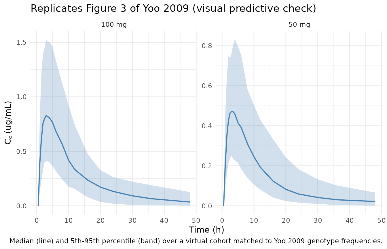
The typical concentration-time curve by CYP3A5 + CYP2C19 genotype combination (zeroed random effects) illustrates the linear-fractional covariate equation. At the 1/1 + EM reference, CL/F is 12.8 L/h; the lowest-clearance combination (3/3 + PM) collapses to 12.8 * (1 - 0.407 - 0.272) = 4.11 L/h.
genotype_grid <- tidyr::expand_grid(
  cyp3a5  = names(cyp3a5_freq),
  cyp2c19 = names(cyp2c19_freq),
  dose_mg = c(50L, 100L)
) |>
  dplyr::mutate(
    id               = dplyr::row_number(),
    treatment        = paste0(dose_mg, " mg"),
    genotype_label   = paste0("CYP3A5 ", cyp3a5, " / CYP2C19 ", cyp2c19),
    CYP3A5_STAR1_HET = as.integer(cyp3a5  == "*1/*3"),
    CYP3A5_STAR1_HOM = as.integer(cyp3a5  == "*1/*1"),
    CYP2C19_IM       = as.integer(cyp2c19 == "IM"),
    CYP2C19_PM       = as.integer(cyp2c19 == "PM")
  )

ev_typ <- genotype_grid |>
  dplyr::group_by(id) |>
  dplyr::reframe(
    dose_mg          = dose_mg[1],
    treatment        = treatment[1],
    genotype_label   = genotype_label[1],
    cyp3a5           = cyp3a5[1],
    cyp2c19          = cyp2c19[1],
    CYP3A5_STAR1_HET = CYP3A5_STAR1_HET[1],
    CYP3A5_STAR1_HOM = CYP3A5_STAR1_HOM[1],
    CYP2C19_IM       = CYP2C19_IM[1],
    CYP2C19_PM       = CYP2C19_PM[1],
    time             = c(0, obs_times),
    evid             = c(1L, rep(0L, length(obs_times))),
    amt              = c(dose_mg[1], rep(0, length(obs_times))),
    cmt              = c("depot", rep("(obs)", length(obs_times)))
  ) |>
  dplyr::ungroup()

sim_geno <- rxode2::rxSolve(
  mod_typ, events = ev_typ,
  keep = c("treatment", "genotype_label", "cyp3a5", "cyp2c19", "dose_mg")
) |> as.data.frame() |>
  dplyr::filter(time > 0)
#> ℹ omega/sigma items treated as zero: 'etalvc', 'etalq', 'etalvp', 'etalcl'
#> Warning: multi-subject simulation without without 'omega'

ggplot(sim_geno, aes(time, Cc, color = cyp3a5, linetype = cyp2c19)) +
  geom_line(linewidth = 0.6) +
  facet_wrap(~treatment) +
  labs(x = "Time (h)", y = expression(C[c] ~ "(ug/mL)"),
       color = "CYP3A5",
       linetype = "CYP2C19",
       title = "Typical curves by CYP3A5 + CYP2C19 genotype combination",
       caption = "Random effects zeroed. Lower clearance shifts the peripheral redistribution and prolongs exposure.") +
  theme_minimal()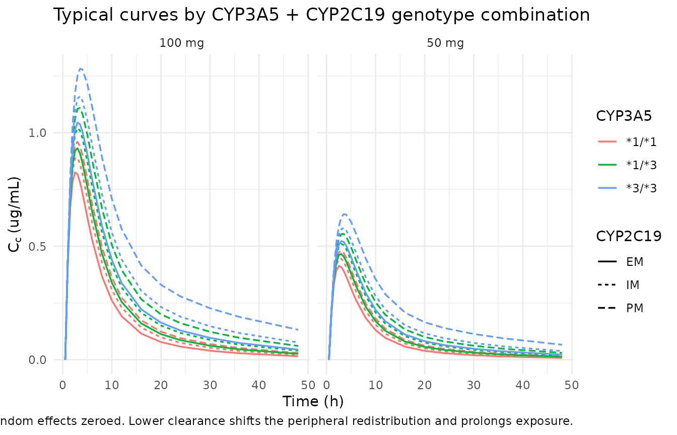
PKNCA validation
Yoo 2009 does not tabulate non-compartmental Cmax / Tmax / AUC / t1/2
values directly. The final model’s linear-fractional CL/F equation
however permits a strict structural cross-check: at the 1/1 +
EM reference, AUC0-infinity should equal dose / (CL/F) =
50 / 12.8 = 3.906 hug/mL at the 50 mg dose and
100 / 12.8 = 7.812 hug/mL at the 100 mg dose. The
PKNCA workflow below computes Cmax, Tmax, AUC0-infinity, AUClast and
terminal half- life on the typical-value (zeroRe) simulation at the
reference genotype, then compares AUC against this structural
expectation.
# Typical-value (*1/*1 + EM) reference cohort, one subject per dose group.
ev_ref <- ev_typ |>
  dplyr::filter(cyp3a5 == "*1/*1", cyp2c19 == "EM")

sim_ref <- rxode2::rxSolve(
  mod_typ, events = ev_ref,
  keep = c("treatment", "dose_mg")
) |> as.data.frame()
#> ℹ omega/sigma items treated as zero: 'etalvc', 'etalq', 'etalvp', 'etalcl'
#> Warning: multi-subject simulation without without 'omega'

sim_nca <- sim_ref |>
  dplyr::filter(!is.na(Cc)) |>
  dplyr::select(id, time, Cc, treatment)

# Guarantee a time = 0 row per (id, treatment); extravascular pre-dose Cc = 0.
sim_nca <- dplyr::bind_rows(
  sim_nca,
  sim_nca |> dplyr::distinct(id, treatment) |>
    dplyr::mutate(time = 0, Cc = 0)
) |>
  dplyr::distinct(id, treatment, time, .keep_all = TRUE) |>
  dplyr::arrange(id, treatment, time)

dose_df <- ev_ref |>
  dplyr::filter(evid == 1) |>
  dplyr::select(id, time, amt, treatment)

conc_obj <- PKNCA::PKNCAconc(sim_nca, Cc ~ time | treatment + id,
                             concu = "ug/mL", timeu = "h")
dose_obj <- PKNCA::PKNCAdose(dose_df, amt ~ time | treatment + id,
                             doseu = "mg")

intervals <- data.frame(
  start      = 0,
  end        = Inf,
  cmax       = TRUE,
  tmax       = TRUE,
  aucinf.obs = TRUE,
  auclast    = TRUE,
  half.life  = TRUE
)

nca_res <- PKNCA::pk.nca(PKNCA::PKNCAdata(conc_obj, dose_obj,
                                          intervals = intervals))
Comparison against the structural CL/F-derived AUC
# Structural expectation: AUC0-inf = dose / (CL/F at *1/*1 + EM) = dose / 12.8.
# Tmax and Cmax do not have closed-form analytic targets in the paper, so they
# are left blank in the reference column (the table only flags rows where a
# numeric reference is present).
published <- tibble::tibble(
  treatment = c("50 mg", "100 mg"),
  aucinf.obs = c(50 / 12.8, 100 / 12.8)
)

cmp <- nlmixr2lib::ncaComparisonTable(
  simulated = nca_res,
  reference = published,
  by        = "treatment",
  units     = c(cmax = "ug/mL", aucinf.obs = "h*ug/mL",
                tmax = "h", half.life = "h", auclast = "h*ug/mL"),
  tolerance_pct = 5
)

knitr::kable(
  cmp,
  caption = paste0(
    "Simulated NCA on the typical-value (*1/*1 + EM) reference subject ",
    "vs. the structural expectation AUC0-inf = dose / CL/F = ",
    "dose / 12.8 L/h. Tolerance: 5%. * differs from reference by >5%."
  ),
  align   = c("l", "l", "r", "r", "r")
)| NCA parameter | treatment | Reference | Simulated | % diff |
|---|---|---|---|---|
| AUC0-∞ (obs) (h*ug/mL) | 50 mg | 3.91 | 3.9 | -0.1% |
| AUC0-∞ (obs) (h*ug/mL) | 100 mg | 7.81 | 7.81 | -0.1% |
Per-genotype Cmax and AUC0-infinity
The table below summarises typical-value NCA across the nine CYP3A5 x CYP2C19 genotype combinations at the 100 mg dose. AUC0-inf should track 100 / CL_geno, where CL_geno follows the Yoo 2009 linear-fractional covariate equation.
ev_geno_100 <- ev_typ |> dplyr::filter(dose_mg == 100L)

sim_geno_ref <- rxode2::rxSolve(
  mod_typ, events = ev_geno_100,
  keep = c("treatment", "genotype_label", "cyp3a5", "cyp2c19", "dose_mg")
) |> as.data.frame()
#> ℹ omega/sigma items treated as zero: 'etalvc', 'etalq', 'etalvp', 'etalcl'
#> Warning: multi-subject simulation without without 'omega'

sim_geno_nca <- sim_geno_ref |>
  dplyr::filter(!is.na(Cc)) |>
  dplyr::select(id, time, Cc, genotype_label)

sim_geno_nca <- dplyr::bind_rows(
  sim_geno_nca,
  sim_geno_nca |> dplyr::distinct(id, genotype_label) |>
    dplyr::mutate(time = 0, Cc = 0)
) |>
  dplyr::distinct(id, genotype_label, time, .keep_all = TRUE) |>
  dplyr::arrange(id, genotype_label, time)

dose_geno_df <- ev_geno_100 |>
  dplyr::filter(evid == 1) |>
  dplyr::select(id, time, amt, genotype_label)

conc_geno <- PKNCA::PKNCAconc(sim_geno_nca,
                              Cc ~ time | genotype_label + id,
                              concu = "ug/mL", timeu = "h")
dose_geno <- PKNCA::PKNCAdose(dose_geno_df,
                              amt ~ time | genotype_label + id,
                              doseu = "mg")

intervals_geno <- data.frame(
  start      = 0,
  end        = Inf,
  cmax       = TRUE,
  tmax       = TRUE,
  aucinf.obs = TRUE
)

nca_geno <- PKNCA::pk.nca(PKNCA::PKNCAdata(conc_geno, dose_geno,
                                            intervals = intervals_geno))

nca_geno_tbl <- as.data.frame(nca_geno$result) |>
  dplyr::filter(PPTESTCD %in% c("cmax", "tmax", "aucinf.obs")) |>
  dplyr::select(genotype_label, PPTESTCD, PPORRES) |>
  tidyr::pivot_wider(names_from = PPTESTCD, values_from = PPORRES) |>
  dplyr::mutate(
    cl_expected = 12.8 * (1 +
                          -0.223 * as.integer(grepl("\\*1/\\*3", genotype_label)) +
                          -0.407 * as.integer(grepl("\\*3/\\*3", genotype_label)) +
                          -0.147 * as.integer(grepl("CYP2C19 IM", genotype_label)) +
                          -0.272 * as.integer(grepl("CYP2C19 PM", genotype_label))),
    auc_expected = 100 / cl_expected
  ) |>
  dplyr::select(`Genotype combination`  = genotype_label,
                `Cmax (ug/mL)`          = cmax,
                `Tmax (h)`              = tmax,
                `AUC0-inf (h*ug/mL)`    = aucinf.obs,
                `Expected CL/F (L/h)`   = cl_expected,
                `Expected AUC (h*ug/mL)` = auc_expected) |>
  dplyr::mutate(dplyr::across(c(`Cmax (ug/mL)`, `Tmax (h)`,
                                `AUC0-inf (h*ug/mL)`,
                                `Expected CL/F (L/h)`,
                                `Expected AUC (h*ug/mL)`),
                              ~ round(., 3)))

knitr::kable(
  nca_geno_tbl,
  caption = paste0(
    "Per-genotype NCA on the typical-value simulation at the 100 mg ",
    "dose. The `Expected CL/F` column reproduces Yoo 2009 final-model ",
    "linear-fractional covariate equation; `Expected AUC` is dose / ",
    "Expected CL/F."
  )
)| Genotype combination | Cmax (ug/mL) | Tmax (h) | AUC0-inf (h*ug/mL) | Expected CL/F (L/h) | Expected AUC (h*ug/mL) |
|---|---|---|---|---|---|
| CYP3A5 1/1 / CYP2C19 EM | 0.825 | 2.5 | 7.808 | 12.800 | 7.812 |
| CYP3A5 1/1 / CYP2C19 IM | 0.890 | 3.0 | 9.154 | 10.918 | 9.159 |
| CYP3A5 1/1 / CYP2C19 PM | 0.960 | 3.0 | 10.725 | 9.318 | 10.731 |
| CYP3A5 1/3 / CYP2C19 EM | 0.932 | 3.0 | 10.049 | 9.946 | 10.055 |
| CYP3A5 1/3 / CYP2C19 IM | 1.021 | 3.0 | 12.392 | 8.064 | 12.401 |
| CYP3A5 1/3 / CYP2C19 PM | 1.109 | 3.5 | 15.454 | 6.464 | 15.470 |
| CYP3A5 3/3 / CYP2C19 EM | 1.045 | 3.0 | 13.164 | 7.590 | 13.175 |
| CYP3A5 3/3 / CYP2C19 IM | 1.160 | 3.5 | 17.494 | 5.709 | 17.517 |
| CYP3A5 3/3 / CYP2C19 PM | 1.282 | 3.5 | 24.278 | 4.109 | 24.338 |
Assumptions and deviations
- Genotype frequencies are sampled independently for CYP3A5 and CYP2C19 in the virtual cohort because Yoo 2009 does not report the joint distribution. Independence is a reasonable default given the two loci are on different chromosomes (CYP3A5 on 7q21.1, CYP2C19 on 10q23.33) and were independently genotyped (Methods ‘Genotype analysis’).
- CYP3A5 indicators are encoded with the canonical paired binaries
CYP3A5_STAR1_HETandCYP3A5_STAR1_HOM(registered ininst/references/covariate-columns.md). The 3/3 stratum that Yoo 2009 uses as the “mutant-type” group is derived insidemodel()as1 - CYP3A5_STAR1_HET - CYP3A5_STAR1_HOMso the linear-fractional CL/F equation reproduces Methods ‘Covariates analysis’ exactly, with no change to the dataset’s covariate columns. - The final-model OMEGA BLOCK reports three off-diagonal covariances
(Vp/F-CL/F, Q/F-Vc/F, Vp/F-Q/F) but not the three remaining
off-diagonals (CL/F-Vc/F, CL/F-Q/F, Vc/F-Vp/F). The model file holds the
unreported off-diagonals at
fixed(0), consistent with standard NONMEM practice of dropping non-significant correlations to zero during stepwise OMEGA-BLOCK building. - Yoo 2009 reports IIV as variance on the eta scale; the paper’s
Discussion quotes
sqrt(omega^2)directly as the CV (e.g., “108% for Q/F and 82.9% for V3/F”). The model file’s omega values are the paper’s reported variances and are not re-derived vialog(1 + CV^2). - Yoo 2009 does not tabulate non-compartmental Cmax / Tmax / AUC /
t1/2 values. The PKNCA comparison uses the structural identity
AUC0-inf = dose / CL/F(at the 1/1 + EM reference, CL/F = 12.8 L/h) as the validation target for AUC; Cmax and Tmax are reported for completeness but have no analytic reference column. - Bioavailability F is not separately identifiable from oral data and
is folded into CL/F, Vc/F, Q/F, Vp/F per the apparent-clearance
convention; the model file therefore does not declare an
lfdepotparameter. - Print-issue year vs DOI year: Br J Clin Pharmacol assigned this
paper to the January 2010 print issue (volume 69, issue 1, pages 27-37),
but the DOI year prefix (
j.1365-2125.2009.03558.x) and the online publication date (4 December 2009) place it as a 2009 paper. The model file uses 2009 to match the task metadata, the DOI year, and the dispatch branch name; the full print citation including the 2010 issue is preserved in thereferencefield for unambiguous bibliographic lookup.