Tripegfilgrastim (Lee 2023)
Source:vignettes/articles/Lee_2023_tripegfilgrastim.Rmd
Lee_2023_tripegfilgrastim.RmdModel and source
mod <- rxode2::rxode(readModelDb("Lee_2023_tripegfilgrastim"))
#> ℹ parameter labels from comments will be replaced by 'label()'- Citation: Lee S, Hong KT, Jang I-J, Yu K-S, Kang HJ, Oh J. (2023). Semimechanistic pharmacokinetic-pharmacodynamic model of tripegfilgrastim for pediatric patients after chemotherapy. CPT Pharmacometrics Syst Pharmacol 12(9):1319-1334. doi:10.1002/psp4.13012.
- Article: https://doi.org/10.1002/psp4.13012
- Description: Semi-mechanistic population PK/PD model for tripegfilgrastim (a PEGylated long-acting recombinant human G-CSF) and absolute neutrophil count (ANC) in healthy Korean adults and Korean pediatric patients with solid tumors receiving chemotherapy. Subcutaneous drug enters a depot compartment and is absorbed at first-order rate KSC into a total-drug compartment. Pharmacodynamics-mediated drug disposition (PDMDD) uses a quasi-equilibrium quadratic between total drug and the circulating G-CSF-receptor pool, giving free drug (FDC) and bound complex (RDC). Free drug is cleared linearly (CLD/VD) and bound drug is internalised (KINT). Granulopoiesis is a five-state receptor chain (stem -> mitotic -> post-mitotic I -> post-mitotic II -> circulating blood receptors) with baselines KP/KTR and KP/KC; ANC = 1000 * RB / SR. Drug binding stimulates receptor production (ST1 = 1 + STM1driver) and bone-marrow transit (ST2 = 1 + STM2driver), where the driver is the fraction of receptors bound by exogenous drug plus endogenous G-CSF. Endogenous G-CSF is carried as its own turnover compartment (fixed KIN, KEL, GCSF0 from Quartino 2014) and a negative-feedback term FB = (RB0/RB)^GAM modulates receptor production. Chemotherapy is a KPD virtual compartment with lag LAG; its output (KCHM*CHM) scaled by CHMSL adds to the mitotic-cell elimination rate. Study population (DIS_HEALTHY) shifts VD and KD, age scales KSC (exponent -0.97, reference 18.5 y), body weight scales KINT (exponent 1.7, reference 55.1 kg), and baseline ANC scales KP (exponential, reference 2106 cells/uL).
Tripegfilgrastim is a PEGylated long-acting recombinant human G-CSF
in which a 23 kDa methoxy-polyethylene-glycol N-hydroxy-succinimide
moiety is conjugated at one of three positions (Lys35, Met N-terminal,
Lys17). Lee 2023 fits a single joint PK-PD model to pooled data from a
healthy adult study (NCT00959777) and a pediatric solid-tumor study
(NCT02963389). The structural framework – quasi-equilibrium
pharmacodynamics-mediated drug disposition (PDMDD) coupled to a
five-state granulopoiesis receptor chain, plus a kinetic-PD (KPD)
chemotherapy compartment – is inherited from Melhem 2018, which is also
in this library as Melhem_2018_g_csf.
Population
str(mod$population, vec.len = 2)
#> List of 11
#>  $ species       : chr "human"
#>  $ n_subjects    : int 67
#>  $ n_studies     : int 2
#>  $ age_range     : chr "6-38 years overall; healthy adults 24 (20-38) years, pediatric patients 12 (6-17) years (median (min-max), Table 1)"
#>  $ weight_range  : chr "18-75 kg overall; healthy adults 69.7 (60-75) kg, pediatric patients 43 (18-67) kg (median (min-max), Table 1)"
#>  $ sex_female_pct: num 11.9
#>  $ race_ethnicity: chr "Korean"
#>  $ disease_state : chr "Two pooled populations: (i) 40 healthy Korean adult male volunteers receiving single subcutaneous tripegfilgras"| __truncated__
#>  $ dose_range    : chr "Healthy adults: single SC tripegfilgrastim 1.8, 3.6, 6 and 18 mg (equivalent to 30, 60, 100 and 300 ug/kg), plu"| __truncated__
#>  $ regions       : chr "Republic of Korea (Seoul National University Hospital)"
#>  $ notes         : chr "Trial registrations NCT00959777 (healthy adults, Ahn 2013) and NCT02963389 (pediatric patients, Lee 2022). 876 "| __truncated__
Lee 2023 Table 1 reports the demographics reproduced below. Note that
the two cohorts are completely separated on age and on chemotherapy
exposure: every healthy participant is an adult male aged 20-38, and
every patient is a pediatric solid-tumor patient aged 6-17 who received
chemotherapy. The DIS_HEALTHY covariate therefore carries a
confounded contrast (see Assumptions and deviations).
tibble::tibble(
  Characteristic = c("n", "Male, n (%)", "Age, y", "Weight, kg",
                     "Height, cm", "BMI, kg/m^2", "BSA, m^2",
                     "Baseline ANC, /uL"),
  `Healthy adults` = c("40", "40 (100)", "24 (20-38)", "69.7 (60-75)",
                       "176 (164-184)", "22.33 (19.37-25.05)",
                       "1.84 (1.67-1.94)", "2607 (1430-5602)"),
  `Pediatric patients` = c("27", "19 (70.4)", "12 (6-17)", "43 (18-67)",
                           "155 (113-178)", "17.94 (13.15-29.76)",
                           "1.39 (0.76-1.79)", "1274 (408-4611)"),
  `Total` = c("67", "59 (88.1)", "22 (6-38)", "64.4 (18-75)",
              "173 (113-184)", "21.12 (13.15-29.76)",
              "1.76 (0.76-1.94)", "2411 (408-5602)")
) |>
knitr::kable(caption = "Lee 2023 Table 1. Median (min-max) unless noted.")| Characteristic | Healthy adults | Pediatric patients | Total |
|---|---|---|---|
| n | 40 | 27 | 67 |
| Male, n (%) | 40 (100) | 19 (70.4) | 59 (88.1) |
| Age, y | 24 (20-38) | 12 (6-17) | 22 (6-38) |
| Weight, kg | 69.7 (60-75) | 43 (18-67) | 64.4 (18-75) |
| Height, cm | 176 (164-184) | 155 (113-178) | 173 (113-184) |
| BMI, kg/m^2 | 22.33 (19.37-25.05) | 17.94 (13.15-29.76) | 21.12 (13.15-29.76) |
| BSA, m^2 | 1.84 (1.67-1.94) | 1.39 (0.76-1.79) | 1.76 (0.76-1.94) |
| Baseline ANC, /uL | 2607 (1430-5602) | 1274 (408-4611) | 2411 (408-5602) |
Source trace
Per-parameter provenance is recorded as an in-file comment next to
each ini() entry in
inst/modeldb/specificDrugs/Lee_2023_tripegfilgrastim.R. The
table below gathers the key entries in one place for review. “Appendix
S1” refers to the Monolix (MLXTRAN) model code supplied as Supporting
Information Text S1.
| Equation / parameter | Value | Source location |
|---|---|---|
Fsc (SC bioavailability) |
1 (Fixed) | Table 2; Results (“bioavailability … was fixed to 1”) |
Ksc (SC absorption rate) |
0.027 /h | Table 2 (RSE 6.1%) |
| beta_Ksc (AGE / 18.5 y) | -0.97 | Table 2 (RSE 13.4%); Equation 7 |
Vd/F healthy adults |
4.7 L | Table 2 (RSE 9.2%); Equation 4 |
Vd/F pediatric patients |
12.7 L | Table 2 (RSE 9.2%); Equation 4 |
CL/F (linear apparent clearance) |
0.18 L/h | Table 2 (RSE 10.8%) |
Kd healthy adults |
42.2 ug/L | Table 2 (RSE 26.7%); Equation 5 |
Kd pediatric patients |
16.2 ug/L | Table 2 (RSE 26.7%); Equation 5 |
Kint (internalisation rate) |
0.41 /h | Table 2 (RSE 15%) |
| beta_Kint (WT / 55.1 kg) | 1.7 | Table 2 (RSE 20.5%); Equation 6 |
Kp (receptor production rate) |
0.083 ug/L/h | Table 2 (RSE 14.4%) |
| beta_Kp (NEUT / 2106 cells/uL) | 0.56 | Table 2 (RSE 13.1%); Equation 8 |
Ktr (bone-marrow transit rate) |
0.033 /h (Fixed) | Table 2; Methods (5-day maturation, refs 13, 28) |
Kc (blood neutrophil elimination) |
0.1155 /h (Fixed) | Appendix S1 code comment; Methods reports 0.116; Table 2 rounds to 0.12 |
Scale / SR (receptor-to-ANC scaling) |
0.54 g per 10^9 cells | Table 2 (RSE 8.5%) |
STM1 (receptor-production stimulation) |
14.4 | Table 2 (RSE 13.5%) |
STM2 (transit-rate stimulation) |
13.8 | Table 2 (RSE 7.4%) |
Gamma (ANC feedback exponent) |
0.145 (Fixed) | Results (ref 32); Table 2 rounds to 0.15 |
GCSF0 (endogenous G-CSF baseline) |
0.0243 ug/L (Fixed) | Results (ref 27 Quartino 2014); Table 2 rounds to 0.024 |
Kel (endogenous G-CSF elimination) |
0.592 /h (Fixed) | Results (ref 27); Table 2 rounds to 0.59 |
Kin (endogenous G-CSF production) |
0.498 ug/L/h (Fixed) | Results (ref 27); Table 2 rounds to 0.5 |
Lag (chemotherapy effect lag) |
171 h | Table 2 (RSE 12.4%) |
Kchemo (chemotherapy KPD decay) |
0.072 /h (Fixed) | Table 2; fixed to Melhem 2018 (ref 23), which reports 0.0724 |
CHMslope (chemo -> mitotic loss slope) |
668 /mg (Fixed) | Table 2; fixed to Melhem 2018 (ref 23), which also reports 668 |
| Omega Ksc / Vd/F / CL/F / Kp | 0.39 / 0.39 / 0.5 / 0.17 | Table 2 Random effects (log-scale SDs) |
| Omega Kd / STM1 / STM2 / Kint | 1.3 / 0.67 / 0.11 / 0.56 | Table 2 Random effects |
| Omega Lag / Kchemo / CHMslope | 0.57 / 0.26 (Fixed) / 2.3 (Fixed) | Table 2 Random effects; Results (Kchemo, CHMslope IIV fixed) |
a1 (PK additive residual) |
0.005 ug/L | Table 2 (RSE 27%) |
b1 (PK proportional residual) |
0.37 | Table 2 (RSE 3.8%) |
a2 (ANC residual, log domain) |
0.48 | Table 2 (RSE 3.1%) |
| Free-drug quadratic FDC | 0.5*(q + sqrt(q^2 + 4 Kd TDC)) |
Appendix S1 EQUATION block |
| Endogenous free G-CSF FEC | same quadratic applied to TEC | Appendix S1 EQUATION block |
| ST1 / ST2 stimulation | 1 + STM_i * ((RDC + REC) / TRC) |
Appendix S1 EQUATION block; Results (linear relationship) |
| Chemotherapy mitotic loss | STM = CHMSL * KCHM * CHM |
Appendix S1 EQUATION block |
| ANC negative feedback | FB = (RB0 / RB)^GAM |
Appendix S1 EQUATION block |
| Granulopoiesis ODE cascade | dSM, dMT, dPM1, dPM2, dRB | Appendix S1 EQUATION block; Figure 1 |
| Initial conditions | SM = MT = PM1 = PM2 = KP/KTR; RB = KP/KC | Appendix S1 EQUATION block |
| Serum concentration observation | CONC = FDC + FEC |
Appendix S1 OUTPUT block |
| ANC observation | ANC = 1000 * RB / SR |
Appendix S1 OUTPUT block |
Covariate-effect verification
The strongest quantitative check available for this model is that the
encoded covariate relationships reproduce, to the digit, the numeric
covariate claims Lee 2023 makes in its Results and Discussion. Each row
below is computed from the model file’s own ini()
values.
th <- mod$theta

ksc_rel <- function(age) (age / 18) ^ th[["e_age_ksc"]]
kp_at   <- function(neut) exp(th[["lkp"]]) * exp(th[["e_neut_kp"]] * neut / 2106)

covariate_check <- tibble::tibble(
  `Paper claim` = c(
    "Ksc ~9-fold higher at age 2 vs age 18",
    "Ksc ~3-fold higher at age 6 vs age 18",
    "Ksc ~40% lower at age 30 vs age 18",
    "Doubling body weight -> ~3-fold higher Kint",
    "Vd/F 4.7 L (healthy) vs 12.7 L (patients)",
    "Kd 62% lower in pediatric patients",
    "Kp = 0.095 ug/L/h at baseline ANC 500/uL",
    "Kp = 0.12 ug/L/h at baseline ANC 1500/uL",
    "Kp doubles from ANC 1500/uL to 4000/uL"
  ),
  `Model value` = c(
    sprintf("%.2f-fold", ksc_rel(2)),
    sprintf("%.2f-fold", ksc_rel(6)),
    sprintf("%.1f%% lower", 100 * (1 - ksc_rel(30))),
    sprintf("%.2f-fold", 2 ^ th[["e_wt_kint"]]),
    sprintf("%.1f L vs %.1f L",
            exp(th[["lvd"]] + th[["e_hv_vd"]]), exp(th[["lvd"]])),
    sprintf("%.0f%% lower",
            100 * (1 - exp(th[["lkd"]]) / exp(th[["lkd"]] + th[["e_hv_kd"]]))),
    sprintf("%.3f ug/L/h", kp_at(500)),
    sprintf("%.3f ug/L/h", kp_at(1500)),
    sprintf("%.2f-fold", kp_at(4000) / kp_at(1500))
  ),
  `Source` = c(
    "Results, 'Population PK-PD model'", "Results, 'Population PK-PD model'",
    "Results, 'Population PK-PD model'", "Discussion (Equation 6)",
    "Results / Table 2 (Equation 4)", "Abstract / Discussion (Equation 5)",
    "Results ('under severe neutropenia states')",
    "Discussion ('when the baseline ANC is 1500/uL')",
    "Discussion ('with a baseline ANC of 4000/uL, the Kp value doubled')"
  )
)
knitr::kable(covariate_check,
caption = "Encoded covariate relationships vs the numeric claims in Lee 2023.")| Paper claim | Model value | Source |
|---|---|---|
| Ksc ~9-fold higher at age 2 vs age 18 | 8.43-fold | Results, ‘Population PK-PD model’ |
| Ksc ~3-fold higher at age 6 vs age 18 | 2.90-fold | Results, ‘Population PK-PD model’ |
| Ksc ~40% lower at age 30 vs age 18 | 39.1% lower | Results, ‘Population PK-PD model’ |
| Doubling body weight -> ~3-fold higher Kint | 3.25-fold | Discussion (Equation 6) |
| Vd/F 4.7 L (healthy) vs 12.7 L (patients) | 4.7 L vs 12.7 L | Results / Table 2 (Equation 4) |
| Kd 62% lower in pediatric patients | 62% lower | Abstract / Discussion (Equation 5) |
| Kp = 0.095 ug/L/h at baseline ANC 500/uL | 0.095 ug/L/h | Results (‘under severe neutropenia states’) |
| Kp = 0.12 ug/L/h at baseline ANC 1500/uL | 0.124 ug/L/h | Discussion (‘when the baseline ANC is 1500/uL’) |
| Kp doubles from ANC 1500/uL to 4000/uL | 1.94-fold | Discussion (‘with a baseline ANC of 4000/uL, the Kp value doubled’) |
Virtual cohort
Two families of scenarios are simulated.
Healthy adults (no chemotherapy). The four single
subcutaneous dose levels of the healthy adult study: 1.8, 3.6, 6 and 18
mg, which the paper states are equivalent to 30, 60, 100 and 300 ug/kg.
Covariates are set to the healthy-adult medians of Table 1 (69.7 kg, 24
years, baseline ANC 2607/uL, DIS_HEALTHY = 1).
Pediatric patients on chemotherapy. The
weight-tiered fixed-dose proposal of Figure 4 / Figure 5 – 1.5, 2.5, 4
and 6 mg for the 10-20, 21-30, 31-44 and >=45 kg bands – each
compared against weight-based 100 ug/kg dosing and against no
tripegfilgrastim at all. Covariates use a representative weight and age
for each band with baseline ANC set to the pediatric median of 1274/uL
and DIS_HEALTHY = 0.
Cohorts are 100 subjects per arm for the stochastic PK cohort and typical-value (zero-IIV) single profiles for the trajectory figures, well inside the 200-per-arm cap.
set.seed(20260730)

# Chemotherapy KPD input. Lee 2023 does not report the mass entered into the
# virtual chemotherapy compartment (16 regimens were pooled), nor the timing of
# that record relative to the tripegfilgrastim dose. See Assumptions and
# deviations for the justification of these two choices.
CHEMO_MG        <- 500
CHEMO_TIME_H    <- 0
DRUG_TIME_CHEMO <- 168   # 24 h after the end of a ~6-day chemotherapy course

make_arm <- function(arm, WT, AGE, NEUT, DIS_HEALTHY,
                     drug_ug, drug_time_h, chemo_mg, obs_grid_h,
                     id_offset = 0L, n = 1L) {
  base_cov <- tibble::tibble(
    id          = id_offset + seq_len(n),
    WT          = WT,
    AGE         = AGE,
    NEUT        = NEUT,
    DIS_HEALTHY = DIS_HEALTHY,
    arm         = arm
  )

  rows <- list()

  if (drug_ug > 0) {
    rows$drug <- base_cov |>
      dplyr::mutate(time = drug_time_h, amt = drug_ug, cmt = "depot",
                    evid = 1L, dvid = NA_integer_)
  }
  if (chemo_mg > 0) {
    rows$chemo <- base_cov |>
      dplyr::mutate(time = CHEMO_TIME_H, amt = chemo_mg,
                    cmt = "depot_kpd_chemotherapy", evid = 1L,
                    dvid = NA_integer_)
  }

  # Observation rows reference the ODE STATE that each algebraic observable is
  # computed from -- Cc from `central` (via the binding quadratic) and ANC from
  # `circ` -- paired with an explicit dvid. Referencing the observables `Cc` /
  # `ANC` directly in `cmt` would inject extra compartment slots.
  obs_grid <- tidyr::expand_grid(base_cov, tibble::tibble(time = obs_grid_h))
  rows$obs_cc  <- obs_grid |>
    dplyr::mutate(amt = NA_real_, cmt = "central", evid = 0L, dvid = 1L)
  rows$obs_anc <- obs_grid |>
    dplyr::mutate(amt = NA_real_, cmt = "circ",    evid = 0L, dvid = 2L)

  dplyr::bind_rows(rows) |>
    dplyr::arrange(id, time, dplyr::desc(evid), dvid)
}
# Healthy adult dose levels (Lee 2023 Methods, 'Data': 1.8, 3.6, 6, 18 mg
# equivalent to 30, 60, 100, 300 ug/kg).
hv_doses <- tibble::tibble(
  arm      = c("HV 1.8 mg (30 ug/kg)", "HV 3.6 mg (60 ug/kg)",
               "HV 6 mg (100 ug/kg)",  "HV 18 mg (300 ug/kg)"),
  drug_ug  = c(1800, 3600, 6000, 18000)
)

obs_grid_hv <- sort(unique(c(seq(0, 336, by = 3), seq(336, 24 * 21, by = 12))))

events_hv <- dplyr::bind_rows(
  lapply(seq_len(nrow(hv_doses)), function(i) {
    make_arm(hv_doses$arm[i], WT = 69.7, AGE = 24, NEUT = 2607,
             DIS_HEALTHY = 1L,
             drug_ug = hv_doses$drug_ug[i], drug_time_h = 0, chemo_mg = 0,
             obs_grid_h = obs_grid_hv, id_offset = (i - 1L) * 10L)
  })
) |>
  dplyr::mutate(arm = factor(arm, levels = hv_doses$arm))
# Weight-tiered fixed doses proposed in Lee 2023 (Simulation / Figure 5) with
# a representative weight and age per band. Ages are chosen to be plausible
# for each weight band (see Assumptions and deviations).
ped_bands <- tibble::tibble(
  band      = c("10-20 kg", "21-30 kg", "31-44 kg", ">=45 kg"),
  WT        = c(15,  25,   37.5, 55),
  AGE       = c(4,   8,    11,   15),
  fixed_ug  = c(1500, 2500, 4000, 6000)
) |>
  dplyr::mutate(wtbased_ug = 100 * WT)

obs_grid_ped <- sort(unique(c(seq(0, 24 * 45, by = 3))))

events_ped <- dplyr::bind_rows(
  lapply(seq_len(nrow(ped_bands)), function(i) {
    b <- ped_bands[i, ]
    dplyr::bind_rows(
      make_arm(paste0(b$band, ": fixed ", b$fixed_ug / 1000, " mg"),
               b$WT, b$AGE, 1274, 0L, b$fixed_ug, DRUG_TIME_CHEMO,
               CHEMO_MG, obs_grid_ped, id_offset = (i - 1L) * 30L + 1L),
      make_arm(paste0(b$band, ": 100 ug/kg"),
               b$WT, b$AGE, 1274, 0L, b$wtbased_ug, DRUG_TIME_CHEMO,
               CHEMO_MG, obs_grid_ped, id_offset = (i - 1L) * 30L + 11L),
      make_arm(paste0(b$band, ": no treatment"),
               b$WT, b$AGE, 1274, 0L, 0, DRUG_TIME_CHEMO,
               CHEMO_MG, obs_grid_ped, id_offset = (i - 1L) * 30L + 21L)
    ) |>
      dplyr::mutate(band = b$band)
  })
) |>
  dplyr::mutate(
    band     = factor(band, levels = ped_bands$band),
    regimen  = dplyr::case_when(
      grepl("fixed", arm)        ~ "Weight-tiered fixed dose",
      grepl("100 ug/kg", arm)    ~ "Weight-based 100 ug/kg",
      TRUE                       ~ "No tripegfilgrastim"
    ),
    regimen  = factor(regimen, levels = c("Weight-tiered fixed dose",
                                          "Weight-based 100 ug/kg",
                                          "No tripegfilgrastim"))
  )
Simulation
Typical-value (zero-IIV) solves pass omega = NA in
addition to using rxode2::zeroRe(). zeroRe()
on its own is not sufficient: once any stochastic rxSolve()
has run in the same R session, rxode2 retains that solve’s
omega and keeps re-sampling etas even though the model’s
own omega matrix is all zeros. The failure is silent and reproducible
under a fixed seed, so a mechanical guard is asserted below.
mod_typical <- rxode2::zeroRe(mod)

sim_hv <- rxode2::rxSolve(
  mod_typical, events = events_hv, omega = NA,
  keep = c("WT", "AGE", "NEUT", "DIS_HEALTHY", "arm"),
  returnType = "data.frame"
) |>
  dplyr::as_tibble()
#> Warning: multi-subject simulation without without 'omega'

sim_ped <- rxode2::rxSolve(
  mod_typical, events = events_ped, omega = NA,
  keep = c("WT", "AGE", "NEUT", "DIS_HEALTHY", "arm", "band", "regimen"),
  returnType = "data.frame"
) |>
  dplyr::as_tibble()
#> Warning: multi-subject simulation without without 'omega'

# Guard: every healthy-adult arm shares the same covariates, so each
# structural parameter must be identical across all of them. If etas were
# being re-sampled these would differ.
stopifnot(
  dplyr::n_distinct(round(sim_hv$vd, 8))   == 1L,
  dplyr::n_distinct(round(sim_hv$cld, 8))  == 1L,
  dplyr::n_distinct(round(sim_hv$kint, 8)) == 1L
)
Baseline verification
With no drug and no chemotherapy the granulopoiesis chain starts at its unstimulated steady state, so ANC(0) = 1000 * (KP / KC) / SR. For a healthy adult with baseline ANC 2607/uL the model’s own baseline should land close to that observed median, and for the pediatric covariate set close to 1274/uL.
baseline <- dplyr::bind_rows(
  sim_hv |> dplyr::filter(time == 0) |>
    dplyr::group_by(Cohort = "Healthy adult (WT 69.7, AGE 24, NEUT 2607)") |>
    dplyr::summarise(`ANC at t = 0 (/uL)` = dplyr::first(ANC),
                     `Free G-CSF at t = 0 (ug/L)` = dplyr::first(Cc),
                     .groups = "drop"),
  sim_ped |> dplyr::filter(time == 0, band == "31-44 kg") |>
    dplyr::group_by(Cohort = "Pediatric patient (WT 37.5, AGE 11, NEUT 1274)") |>
    dplyr::summarise(`ANC at t = 0 (/uL)` = dplyr::first(ANC),
                     `Free G-CSF at t = 0 (ug/L)` = dplyr::first(Cc),
                     .groups = "drop")
)
knitr::kable(baseline, digits = 4,
caption = "Model baseline at t = 0 (paper observed medians: 2607/uL healthy, 1274/uL pediatric).")| Cohort | ANC at t = 0 (/uL) | Free G-CSF at t = 0 (ug/L) |
|---|---|---|
| Healthy adult (WT 69.7, AGE 24, NEUT 2607) | 2661.728 | 0.0050 |
| Pediatric patient (WT 37.5, AGE 11, NEUT 1274) | 1867.352 | 0.0018 |
Replicate published figures
Figure 2a – tripegfilgrastim concentration-time profiles
Lee 2023 Figure 2a (and Figure S3) show prediction-corrected concentration-time profiles across the healthy-adult dose levels. Absorption is slow (Ksc = 0.027 /h) and the decline is dominated by receptor-mediated internalisation, so the profile is markedly non-linear in dose: at low doses the receptor pool absorbs most of the drug, while at 300 ug/kg the receptor pathway saturates and exposure rises more than proportionally.
sim_hv |>
  dplyr::filter(!is.na(Cc), Cc > 0) |>
  dplyr::group_by(arm, time) |>
  dplyr::summarise(Cc = dplyr::first(Cc), .groups = "drop") |>
  ggplot2::ggplot(ggplot2::aes(time / 24, Cc, colour = arm)) +
  ggplot2::geom_line(linewidth = 0.7) +
  ggplot2::scale_y_log10() +
  ggplot2::scale_x_continuous(breaks = seq(0, 14, by = 2), limits = c(0, 14)) +
  ggplot2::labs(x = "Time (days)", y = "Serum tripegfilgrastim (ug/L)",
                colour = NULL,
                title = "Typical-value tripegfilgrastim PK in healthy adults",
                subtitle = "Replicates the shape of Lee 2023 Figure 2a / Figure S3") +
  ggplot2::theme_minimal() +
  ggplot2::theme(legend.position = "bottom")
#> Warning: Removed 56 rows containing missing values or values outside the scale range
#> (`geom_line()`).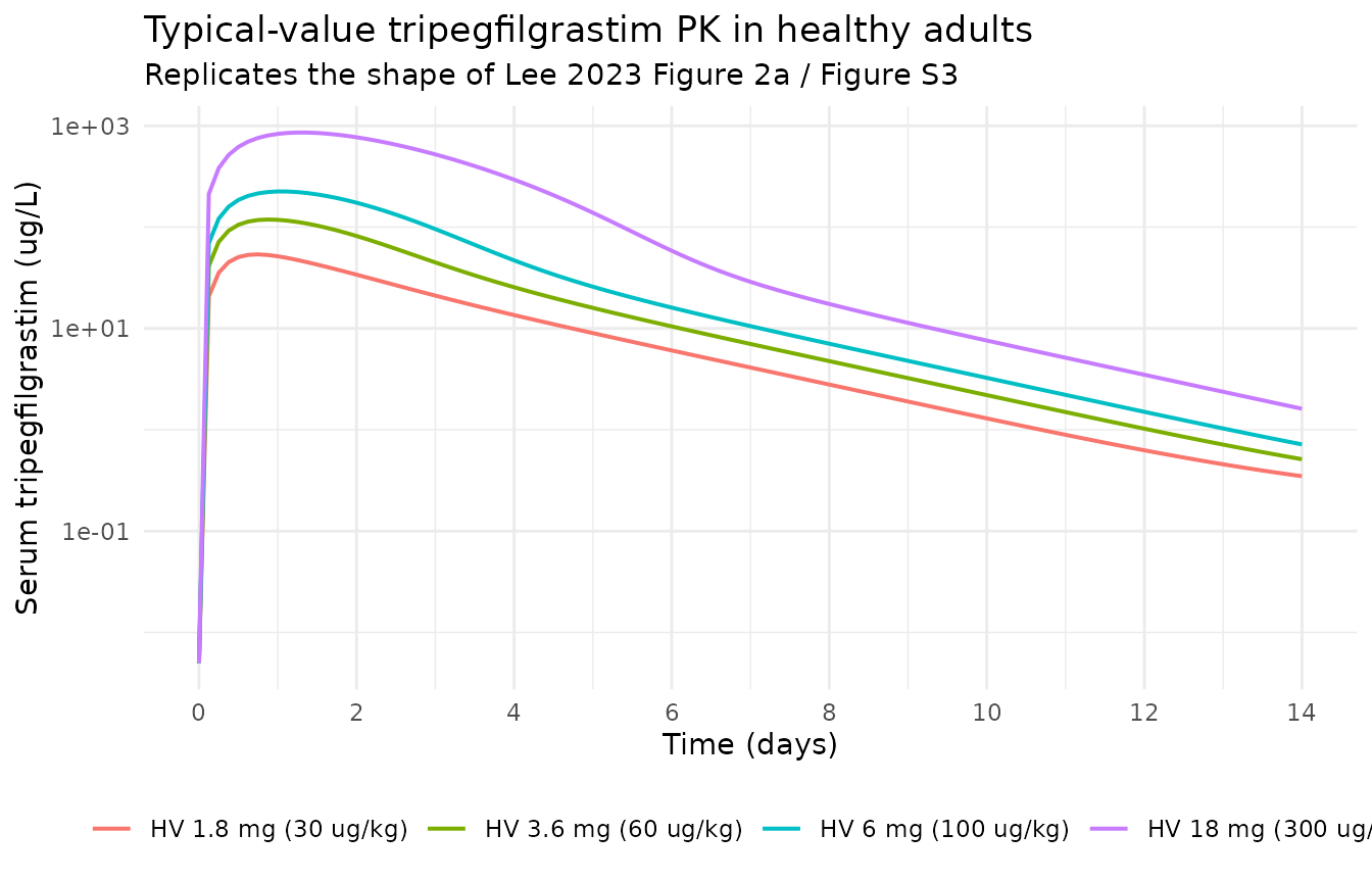
Figure 2b – ANC response in healthy adults
Lee 2023 Figure 2b / Figure S4 show the ANC response. ANC rises sharply within the first day, peaks around days 1-2, and returns toward baseline by roughly day 7 in healthy subjects (Results, “The ANC level recovered to baseline after 7 days in healthy subjects”).
sim_hv |>
  dplyr::filter(!is.na(ANC)) |>
  dplyr::group_by(arm, time) |>
  dplyr::summarise(ANC = dplyr::first(ANC), .groups = "drop") |>
  ggplot2::ggplot(ggplot2::aes(time / 24, ANC, colour = arm)) +
  ggplot2::geom_line(linewidth = 0.7) +
  ggplot2::geom_hline(yintercept = 2607, linetype = "dashed", colour = "grey40") +
  ggplot2::scale_x_continuous(breaks = seq(0, 14, by = 2), limits = c(0, 14)) +
  ggplot2::labs(x = "Time (days)", y = "ANC (cells/uL)", colour = NULL,
                title = "Typical-value ANC response in healthy adults",
                subtitle = "Dashed line = observed median baseline ANC 2607/uL (Lee 2023 Table 1)") +
  ggplot2::theme_minimal() +
  ggplot2::theme(legend.position = "bottom")
#> Warning: Removed 56 rows containing missing values or values outside the scale range
#> (`geom_line()`).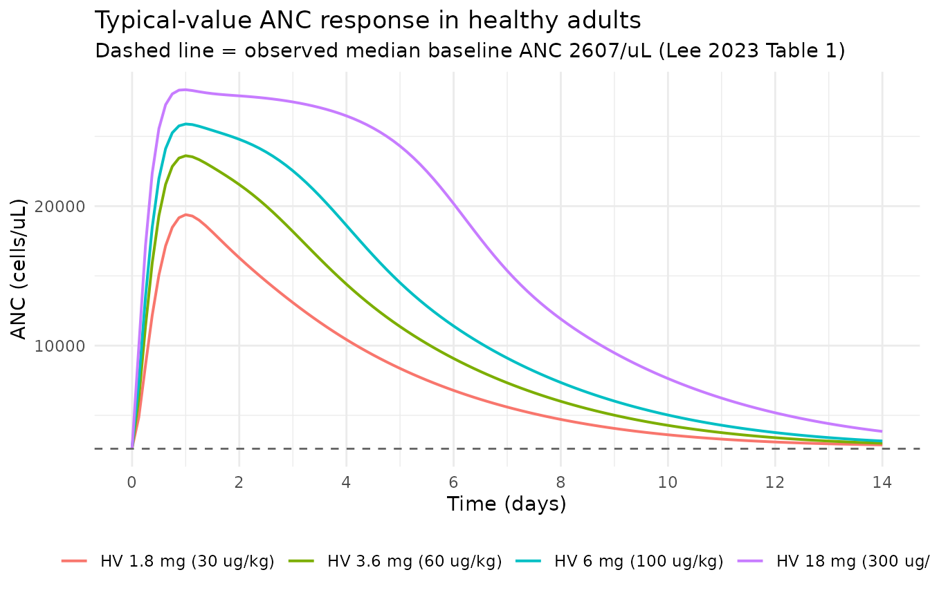
Figure 3 – fractional G-CSF receptor occupancy
Lee 2023 computes fractional receptor occupancy as the free-drug concentration divided by the sum of the free-drug concentration and Kd (Methods, “Simulation”). Because pediatric patients have a 62% lower Kd and a higher Vd/F, the paper reports that patients show a more sustained fractional occupancy than healthy adults (Figure 3).
occ_events <- dplyr::bind_rows(
  make_arm("Healthy adult, 100 ug/kg", 69.7, 24, 2607, 1L,
           100 * 69.7, 0, 0, seq(0, 24 * 14, by = 3), id_offset = 0L),
  make_arm("Pediatric patient, 100 ug/kg", 43, 12, 1274, 0L,
           100 * 43, 0, 0, seq(0, 24 * 14, by = 3), id_offset = 10L)
)

sim_occ <- rxode2::rxSolve(
  mod_typical, events = occ_events, omega = NA,
  keep = c("WT", "AGE", "NEUT", "DIS_HEALTHY", "arm"),
  returnType = "data.frame"
) |>
  dplyr::as_tibble() |>
  dplyr::filter(!is.na(Cc)) |>
  dplyr::group_by(arm, time) |>
  dplyr::summarise(occupancy = dplyr::first(fdc / (fdc + kd)), .groups = "drop")
#> Warning: multi-subject simulation without without 'omega'

ggplot2::ggplot(sim_occ, ggplot2::aes(time / 24, occupancy, colour = arm)) +
  ggplot2::geom_line(linewidth = 0.7) +
  ggplot2::scale_y_continuous(limits = c(0, 1)) +
  ggplot2::labs(x = "Time (days)", y = "Fractional G-CSF receptor occupancy",
                colour = NULL,
                title = "Fractional receptor occupancy after 100 ug/kg",
                subtitle = "Replicates Lee 2023 Figure 3: occupancy is more sustained in patients (lower Kd)") +
  ggplot2::theme_minimal() +
  ggplot2::theme(legend.position = "bottom")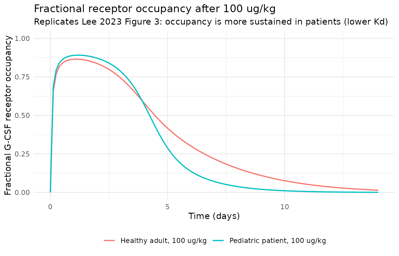
Figure 4 – weight-tiered fixed dosing vs weight-based dosing
Lee 2023 Figure 4 compares ANC-time profiles for the proposed fixed doses against weight-based 100 ug/kg dosing and against no tripegfilgrastim, within each weight band. The paper’s conclusion is that the fixed-dose and weight-based profiles are near-superimposable and both are clearly better than no treatment.
sim_ped |>
  dplyr::filter(!is.na(ANC)) |>
  dplyr::group_by(band, regimen, time) |>
  dplyr::summarise(ANC = dplyr::first(ANC), .groups = "drop") |>
  ggplot2::ggplot(ggplot2::aes(time / 24, ANC, colour = regimen)) +
  ggplot2::geom_line(linewidth = 0.6) +
  ggplot2::geom_hline(yintercept = 500, linetype = "dotted", colour = "grey30") +
  ggplot2::facet_wrap(~band) +
  ggplot2::scale_y_log10() +
  ggplot2::labs(x = "Time (days from chemotherapy)", y = "ANC (cells/uL)",
                colour = NULL,
                title = "Weight-tiered fixed dose vs weight-based 100 ug/kg",
                subtitle = "Replicates the structure of Lee 2023 Figure 4. Dotted line = 500/uL (Grade 4)") +
  ggplot2::theme_minimal() +
  ggplot2::theme(legend.position = "bottom")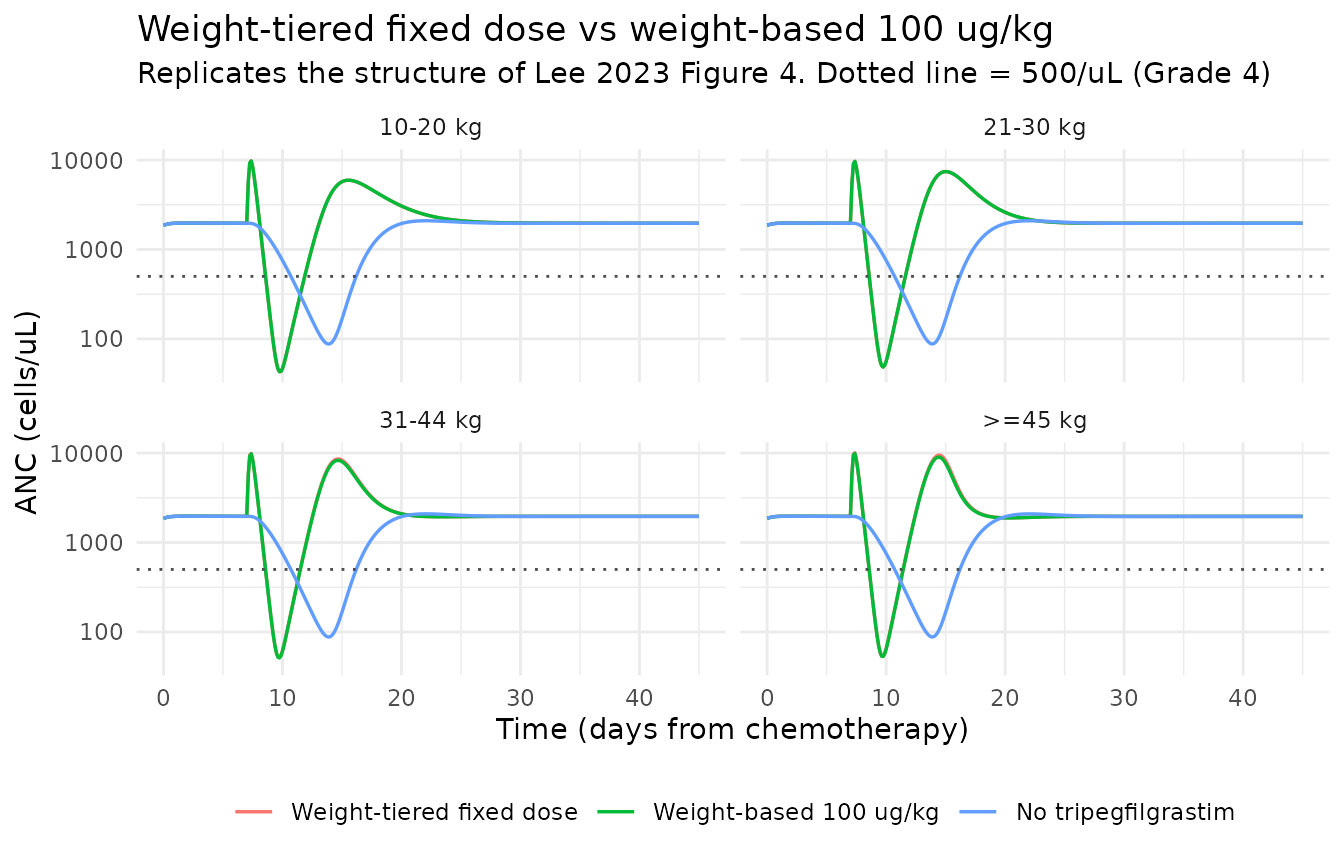
Figure 5 – Grade 4 neutropenia duration
Lee 2023 Figure 5 compares the duration of Grade 4 neutropenia (ANC < 500/uL) across the fixed-dose and weight-based regimens. The paper’s reported medians are 7.0, 6.8, 6.5 and 6.3 days for the fixed doses and 7.2, 7.2, 6.6 and 6.5 days for 100 ug/kg, in the 10-20, 21-30, 31-44 and >=45 kg bands respectively; the untreated control is longer in every band.
grid_h <- 3

g4 <- sim_ped |>
  dplyr::filter(!is.na(ANC)) |>
  dplyr::group_by(band, regimen, time) |>
  dplyr::summarise(ANC = dplyr::first(ANC), .groups = "drop") |>
  dplyr::group_by(band, regimen) |>
  dplyr::summarise(
    `Grade 4 duration (days)` = sum(ANC < 500) * grid_h / 24,
    `ANC nadir (cells/uL)`    = min(ANC),
    `Time to nadir (days)`    = time[which.min(ANC)] / 24,
    .groups = "drop"
  )

knitr::kable(g4, digits = 2,
caption = "Simulated typical-value Grade 4 neutropenia metrics by weight band and regimen.")| band | regimen | Grade 4 duration (days) | ANC nadir (cells/uL) | Time to nadir (days) |
|---|---|---|---|---|
| 10-20 kg | Weight-tiered fixed dose | 3.25 | 42.95 | 9.75 |
| 10-20 kg | Weight-based 100 ug/kg | 3.25 | 42.95 | 9.75 |
| 10-20 kg | No tripegfilgrastim | 5.50 | 87.68 | 13.88 |
| 21-30 kg | Weight-tiered fixed dose | 3.00 | 48.43 | 9.75 |
| 21-30 kg | Weight-based 100 ug/kg | 3.00 | 48.43 | 9.75 |
| 21-30 kg | No tripegfilgrastim | 5.50 | 87.72 | 13.88 |
| 31-44 kg | Weight-tiered fixed dose | 2.88 | 51.69 | 9.75 |
| 31-44 kg | Weight-based 100 ug/kg | 3.00 | 51.29 | 9.75 |
| 31-44 kg | No tripegfilgrastim | 5.50 | 87.78 | 13.88 |
| >=45 kg | Weight-tiered fixed dose | 2.88 | 53.58 | 9.75 |
| >=45 kg | Weight-based 100 ug/kg | 2.88 | 53.15 | 9.75 |
| >=45 kg | No tripegfilgrastim | 5.50 | 87.90 | 13.88 |
ggplot2::ggplot(g4, ggplot2::aes(band, `Grade 4 duration (days)`, fill = regimen)) +
  ggplot2::geom_col(position = ggplot2::position_dodge(width = 0.8), width = 0.7) +
  ggplot2::labs(x = "Weight band", y = "Grade 4 neutropenia duration (days)",
                fill = NULL,
                title = "Grade 4 neutropenia duration by weight band and regimen",
                subtitle = "Replicates the comparison of Lee 2023 Figure 5 (typical-value, single representative subject per band)") +
  ggplot2::theme_minimal() +
  ggplot2::theme(legend.position = "bottom")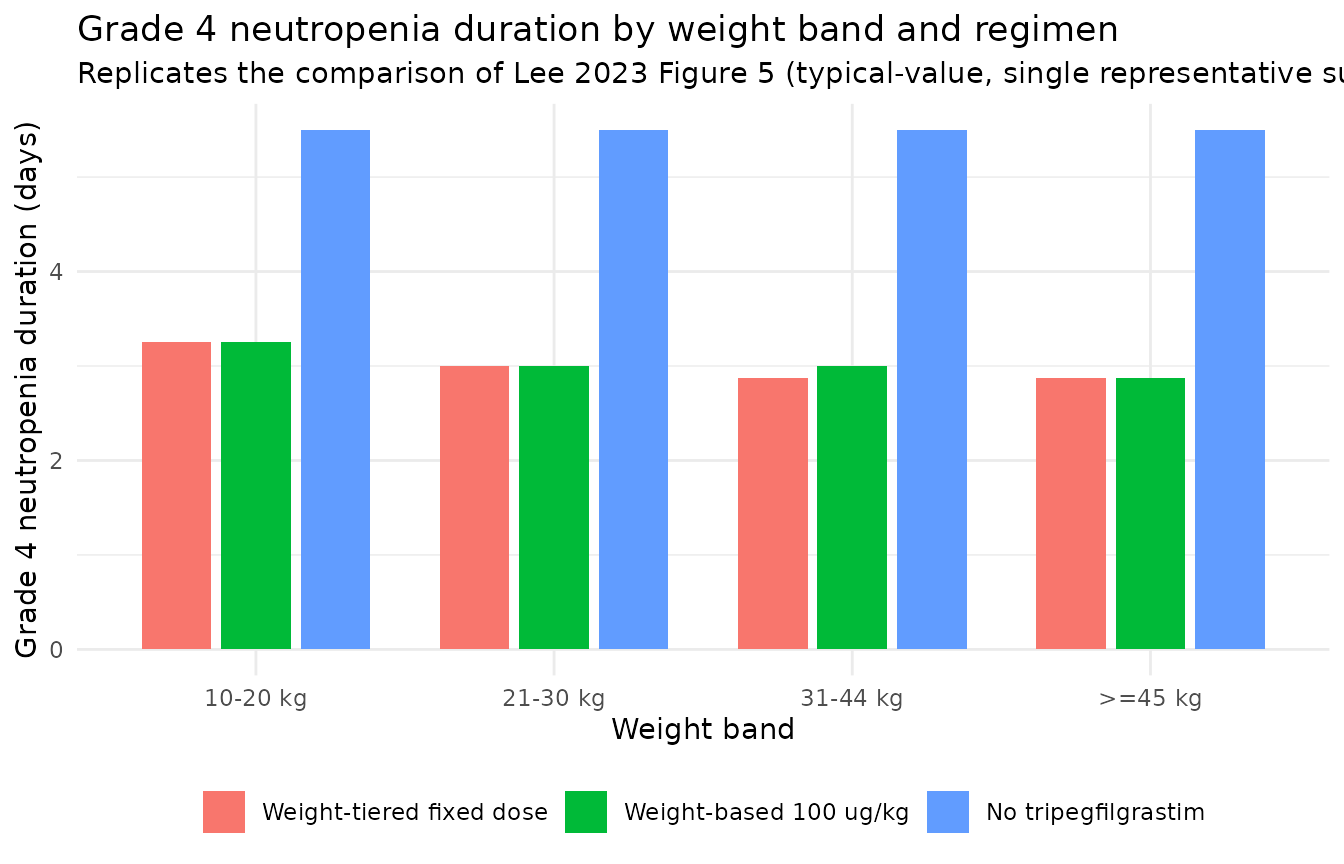
The fixed-dose and weight-based arms track each other closely within every band and both shorten Grade 4 neutropenia relative to no treatment, reproducing the paper’s qualitative conclusion. The absolute durations are shorter than the paper’s medians because these are typical-value (zero-IIV) single subjects, whereas Lee 2023 reports medians over 500 virtual patients that carry the full random-effect distribution – notably Omega_Lag = 0.57 and Omega_Kd = 1.3 – plus parameter uncertainty from the variance-covariance matrix. See Assumptions and deviations for the chemotherapy-input caveat.
PKNCA validation
A stochastic cohort of 100 healthy adults per dose level is simulated with full inter-individual variability and summarised with PKNCA. Lee 2023 does not tabulate NCA parameters, so this section establishes the model’s exposure metrics and checks the dose-proportionality behaviour that the PDMDD structure implies.
n_per_arm <- 100L

events_nca <- dplyr::bind_rows(
  lapply(seq_len(nrow(hv_doses)), function(i) {
    make_arm(hv_doses$arm[i], WT = 69.7, AGE = 24, NEUT = 2607,
             DIS_HEALTHY = 1L,
             drug_ug = hv_doses$drug_ug[i], drug_time_h = 0, chemo_mg = 0,
             obs_grid_h = obs_grid_hv,
             id_offset = (i - 1L) * n_per_arm, n = n_per_arm)
  })
) |>
  dplyr::mutate(arm = factor(arm, levels = hv_doses$arm))

sim_nca <- rxode2::rxSolve(
  mod, events = events_nca,
  keep = c("WT", "AGE", "NEUT", "DIS_HEALTHY", "arm"),
  returnType = "data.frame"
) |>
  dplyr::as_tibble()

# Assert the population simulation returned every requested subject.
stopifnot(dplyr::n_distinct(sim_nca$id) == n_per_arm * nrow(hv_doses))
conc_nca <- sim_nca |>
  dplyr::filter(!is.na(Cc)) |>
  dplyr::group_by(id, arm, time) |>
  dplyr::summarise(Cc = dplyr::first(Cc), .groups = "drop")

# Time-zero records must be present or PKNCA warns about the AUC start.
stopifnot(all(tapply(conc_nca$time, conc_nca$id, min) == 0))

dose_nca <- events_nca |>
  dplyr::filter(cmt == "depot", evid == 1L) |>
  dplyr::select(id, arm, time, amt)

conc_obj <- PKNCA::PKNCAconc(conc_nca, Cc ~ time | arm + id,
                             concu = "ug/L", timeu = "hour")
dose_obj <- PKNCA::PKNCAdose(dose_nca, amt ~ time | arm + id, doseu = "ug")

intervals_nca <- data.frame(
  start      = 0,
  end        = Inf,
  cmax       = TRUE,
  tmax       = TRUE,
  auclast    = TRUE,
  aucinf.obs = TRUE,
  half.life  = TRUE
)

res_nca <- PKNCA::pk.nca(
  PKNCA::PKNCAdata(conc_obj, dose_obj, intervals = intervals_nca)
)
summary(res_nca)
#>  Interval Start Interval End                  arm   N AUClast (hour*ug/L)
#>               0          Inf HV 1.8 mg (30 ug/kg) 100          3040 [122]
#>               0          Inf HV 3.6 mg (60 ug/kg) 100         7660 [93.8]
#>               0          Inf  HV 6 mg (100 ug/kg) 100        14300 [83.9]
#>               0          Inf HV 18 mg (300 ug/kg) 100        53500 [75.9]
#>  Cmax (ug/L)       Tmax (hour)     Half-life (hour) AUCinf,obs (hour*ug/L)
#>  44.9 [85.1] 18.0 [3.00, 60.0] 45000 [183000], n=96       5360 [178], n=96
#>   105 [72.8] 21.0 [3.00, 78.0]  17200 [56700], n=93       9830 [108], n=93
#>   227 [64.4] 21.0 [9.00, 51.0]  29300 [98800], n=96     17700 [97.7], n=96
#>   708 [58.6] 27.0 [9.00, 72.0]   6030 [28400], n=97     54500 [77.6], n=97
#>
#> Caption: AUClast, Cmax, AUCinf,obs: geometric mean and geometric coefficient of variation; Tmax: median and range; Half-life: arithmetic mean and standard deviation; N: number of subjects; n: number of measurements included in summary
Comparison against published values
Lee 2023 reports no NCA table, so the comparison below is against the quantitative statements the paper does make about exposure and response.
nca_med <- as.data.frame(res_nca$result) |>
  dplyr::filter(PPTESTCD %in% c("cmax", "tmax", "aucinf.obs", "half.life")) |>
  dplyr::group_by(arm, PPTESTCD) |>
  dplyr::summarise(value = median(PPORRES, na.rm = TRUE), .groups = "drop")

dose_prop <- nca_med |>
  dplyr::filter(PPTESTCD %in% c("cmax", "aucinf.obs")) |>
  dplyr::left_join(hv_doses, by = "arm") |>
  dplyr::group_by(PPTESTCD) |>
  dplyr::mutate(
    `Dose ratio vs 1.8 mg`     = drug_ug / min(drug_ug),
    `Exposure ratio vs 1.8 mg` = value / value[which.min(drug_ug)]
  ) |>
  dplyr::ungroup() |>
  dplyr::select(arm, PPTESTCD, value,
                `Dose ratio vs 1.8 mg`, `Exposure ratio vs 1.8 mg`) |>
  dplyr::rename("Arm" = arm, "NCA parameter" = PPTESTCD,
                "Median simulated value" = value)

knitr::kable(dose_prop, digits = 2,
caption = "Dose proportionality of simulated exposure in healthy adults. More-than-proportional increases reflect saturation of the receptor-mediated elimination pathway.")| Arm | NCA parameter | Median simulated value | Dose ratio vs 1.8 mg | Exposure ratio vs 1.8 mg |
|---|---|---|---|---|
| HV 1.8 mg (30 ug/kg) | aucinf.obs | 4827.16 | 1.00 | 1.00 |
| HV 1.8 mg (30 ug/kg) | cmax | 50.14 | 1.00 | 1.00 |
| HV 3.6 mg (60 ug/kg) | aucinf.obs | 10493.28 | 2.00 | 2.17 |
| HV 3.6 mg (60 ug/kg) | cmax | 117.02 | 2.00 | 2.33 |
| HV 6 mg (100 ug/kg) | aucinf.obs | 17653.45 | 3.33 | 3.66 |
| HV 6 mg (100 ug/kg) | cmax | 239.59 | 3.33 | 4.78 |
| HV 18 mg (300 ug/kg) | aucinf.obs | 55353.35 | 10.00 | 11.47 |
| HV 18 mg (300 ug/kg) | cmax | 746.94 | 10.00 | 14.90 |
Lee 2023 Figure S5 contrasts healthy subjects against chemotherapy
patients within the same age group, so the comparison
below holds weight and age fixed and varies only
DIS_HEALTHY. That isolates the population effect, which is
carried entirely by Vd/F (4.7 vs 12.7 L) and Kd (42.2 vs 16.2 ug/L).
# These typical-value solves run AFTER the stochastic PKNCA cohort above, so
# omega = NA is load-bearing here (see the note in the Simulation section).
run_matched <- function(WT, AGE, healthy, tmax_h = 24 * 21) {
  ev <- make_arm(if (healthy) "Healthy" else "Patient",
                 WT, AGE, 1274, as.integer(healthy),
                 100 * WT, 0, 0, seq(0, tmax_h, by = 3))
  rxode2::rxSolve(mod_typical, events = ev, omega = NA,
                  keep = c("WT", "AGE", "NEUT", "DIS_HEALTHY", "arm"),
                  returnType = "data.frame")
}

matched <- lapply(list(c(4, 15), c(9, 28), c(15, 50)), function(ag) {
  hv <- run_matched(ag[2], ag[1], TRUE)
  pt <- run_matched(ag[2], ag[1], FALSE)
  tibble::tibble(
    `Age (y) / weight (kg)` = sprintf("%d / %d", ag[1], ag[2]),
    `Cmax healthy (ug/L)`   = max(hv$Cc),
    `Cmax patient (ug/L)`   = max(pt$Cc),
    `Ratio`                 = max(hv$Cc) / max(pt$Cc)
  )
}) |>
  dplyr::bind_rows()

knitr::kable(matched, digits = c(0, 0, 0, 2),
caption = "Peak concentration after 100 ug/kg, healthy vs chemotherapy patient at matched age and weight. Lee 2023 Results describes this ratio as approximately three-fold.")| Age (y) / weight (kg) | Cmax healthy (ug/L) | Cmax patient (ug/L) | Ratio |
|---|---|---|---|
| 4 / 15 | 178 | 78 | 2.30 |
| 9 / 28 | 242 | 109 | 2.22 |
| 15 / 50 | 316 | 128 | 2.47 |
occ_matched <- dplyr::bind_rows(
  run_matched(43, 12, TRUE)  |> dplyr::mutate(pop = "Healthy"),
  run_matched(43, 12, FALSE) |> dplyr::mutate(pop = "Patient")
) |>
  dplyr::filter(time %in% (c(1, 2, 3, 5, 7, 10, 14) * 24)) |>
  dplyr::group_by(pop, time) |>
  dplyr::summarise(occupancy = dplyr::first(fdc / (fdc + kd)), .groups = "drop") |>
  tidyr::pivot_wider(names_from = pop, values_from = occupancy) |>
  dplyr::mutate(Day = time / 24) |>
  dplyr::select(Day, Healthy, Patient)

knitr::kable(occ_matched, digits = 3,
caption = "Fractional G-CSF receptor occupancy at matched age (12 y) and weight (43 kg) after 100 ug/kg. Occupancy is higher in patients at every time point and the relative gap widens as drug is cleared, reproducing the more sustained occupancy Lee 2023 reports in Figure 3.")| Day | Healthy | Patient |
|---|---|---|
| 1 | 0.881 | 0.890 |
| 2 | 0.839 | 0.872 |
| 3 | 0.717 | 0.787 |
| 5 | 0.277 | 0.289 |
| 7 | 0.063 | 0.071 |
| 10 | 0.006 | 0.011 |
| 14 | 0.000 | 0.001 |
hv_adult <- rxode2::rxSolve(
  mod_typical, omega = NA,
  events = make_arm("HV adult", 69.7, 24, 2607, 1L, 100 * 69.7, 0, 0,
                    seq(0, 24 * 21, by = 3)),
  keep = c("WT", "AGE", "NEUT", "DIS_HEALTHY", "arm"),
  returnType = "data.frame"
)

# Guard: the typical-value solve must reproduce the structural typical Vd/F.
stopifnot(isTRUE(all.equal(
  unique(round(hv_adult$vd, 6)),
  round(exp(th[["lvd"]] + th[["e_hv_vd"]]), 6)
)))

anc_bl <- hv_adult$ANC[1]
tibble::tibble(
  Day = c(1, 2, 3, 5, 7, 10, 14, 21),
  `ANC (cells/uL)` = vapply(Day, function(d)
    hv_adult$ANC[which.min(abs(hv_adult$time - d * 24))], numeric(1)),
) |>
  dplyr::mutate(`Fold over baseline` = `ANC (cells/uL)` / anc_bl) |>
  knitr::kable(digits = c(0, 0, 2),
caption = sprintf("Typical-value ANC after 100 ug/kg in a healthy adult (baseline %.0f cells/uL). See Assumptions and deviations regarding the recovery time.", anc_bl))| Day | ANC (cells/uL) | Fold over baseline |
|---|---|---|
| 1 | 26399 | 9.92 |
| 2 | 25494 | 9.58 |
| 3 | 23640 | 8.88 |
| 5 | 15671 | 5.89 |
| 7 | 9724 | 3.65 |
| 10 | 5289 | 1.99 |
| 14 | 3221 | 1.21 |
| 21 | 2798 | 1.05 |
Assumptions and deviations
-
The chemotherapy KPD input is not reported and is a
user-supplied simulation input. Lee 2023 pooled 16 different
chemotherapy regimen combinations and never tabulates the mass entered
into the virtual chemotherapy compartment, nor the time of that dose
record relative to the tripegfilgrastim dose. Both are required to
simulate the pediatric arms. This vignette uses
CHEMO_MG = 500mg at time 0 and gives tripegfilgrastim atDRUG_TIME_CHEMO = 168h. The timing choice follows from the protocol and the model itself: the trial gave tripegfilgrastim 24 h after the end of a multi-day chemotherapy course, and the estimated lag between the chemotherapy dose record and its effect on mitotic cells is Lag = 171 h, so the drug dose and the onset of mitotic kill nearly coincide. If instead the chemotherapy record is placed only 24 h before the drug, the entire ANC-stimulating effect of tripegfilgrastim is spent about six days before the chemotherapy effect emerges, and the model then predicts a longer Grade 4 duration in treated than in untreated subjects – the opposite of the paper’s Figure 5. Users simulating this model must set both the chemotherapy mass and its timing deliberately; neither is recoverable from the publication. The model file itself is unaffected: everyini()parameter is reported by the paper. -
Baseline ANC is model-determined, not forced. The
granulopoiesis chain starts at KP/KTR and KP/KC, so the baseline ANC
follows from KP (which carries the
NEUTcovariate), KC and SR rather than being set to the observed baseline. At the healthy-adult covariate set the model baseline is close to the observed median of 2607/uL; at the pediatric covariate set it sits above the observed median of 1274/uL, because the pediatric median baseline is itself depressed by prior chemotherapy that the covariate model does not represent. -
Endogenous G-CSF is not at steady state at time 0, as
published. Appendix S1 sets
EN_0 = GCSF0(0.0243 ug/L) while the turnover parameters KIN = 0.498 ug/L/h and KEL = 0.592 /h – both fixed to Quartino 2014 – imply a different equilibrium. The endogenous compartment therefore drifts upward over the first few hours to roughly 0.06-0.07 ug/L before settling. The model file reproduces the published code verbatim rather than re-deriving a self-consistent baseline. The practical impact is small: endogenous free G-CSF contributes well under 1% of the observed concentration while drug is present, and adds roughly a 5% baseline offset to the ST1 / ST2 stimulation terms. -
Dimensional inconsistency in the published endogenous
equation. In Appendix S1,
ddt_EN = KIN - KEN*(FEC*VD) - KINT*(REC*VD)mixes a concentration-rate production term (KIN, ug/L/h) with amount-rate loss terms (ug/h). The model file reproduces the equation exactly as printed. Downstream users who need a dimensionally consistent endogenous arm should scale KIN by VD. -
KENis a transcription typo forKEL. The Appendix S1 input block declaresKEL(“non-specific linear elimination rate constant of endogenous G-CSF … fixed to 0.592 h-1”) but the ODE line uses the undeclared symbolKEN. There is only one candidate, so the model file uses KEL = 0.592 /h. - Endogenous and exogenous binding are computed independently, as published. Appendix S1 applies the same quasi-equilibrium quadratic separately to tripegfilgrastim and to endogenous G-CSF, each against the full receptor pool TRC. This is an approximation to competitive binding rather than a solution of it – the two species can jointly occupy more than 100% of the receptor pool in principle. Because endogenous concentrations are three to four orders of magnitude below the exogenous peak, the approximation is numerically inconsequential here. The model file reproduces the published formulation.
- Fixed parameters are reported at their most precise published value. Where Table 2 rounds a fixed parameter that the Methods, Results or Appendix S1 report more precisely, the model file uses the more precise value and records both: KC = 0.1155 /h (Appendix S1; Methods 0.116; Table 2 0.12), GAM = 0.145 (Results; Table 2 0.15), GCSF0 = 0.0243 ug/L (Results; Table 2 0.024), KEL = 0.592 /h (Results; Table 2 0.59), KIN = 0.498 ug/L/h (Results; Table 2 0.5). KCHM and CHMSL are kept at Lee 2023’s own printed 0.072 /h and 668 /mg; the upstream Melhem 2018 values they were fixed to are 0.0724 /h and 668 /mg.
-
Omega values are log-scale SDs. Lee 2023 Table 2’s
“Random effects” rows are standard deviations, not variances. This is
confirmed independently by the Results text, which reports the Lag IIV
as 62.6% CV: sqrt(exp(0.57^2) - 1) = 0.626. The nlmixr2
ini()block stores variances, so each entry is squared. -
IIV on Kchemo and CHMslope is fixed. Lee 2023
Results states that “Random effects were all estimated except for Kchemo
and CHMslope, which were fixed with the reported value”, and Table 2
reports those two rows without RSE or bootstrap columns. They are
encoded with
fixed(). Lee 2023 does not report a correlation between them, unlike Melhem 2018 (r = 0.731), so they are encoded as independent. -
PK residual error is combined additive plus
proportional. The paper reports a1 = 0.005 ug/L and b1 = 0.37
but does not state whether Monolix’s
combined1(a + bf) orcombined2(sqrt(a^2 + (bf)^2)) form was used. The model file uses nlmixr2’s standardprop() + add(), which is thecombined2form. Because a1 is four orders of magnitude below typical simulated concentrations, the two forms are numerically indistinguishable here. -
DIS_HEALTHYis a confounded contrast. In this analysis the indicator separates healthy adult males aged 20-38 from pediatric solid-tumor patients aged 6-17 who received chemotherapy, so it conflates health status, age stratum and chemotherapy exposure. The paper acknowledges this as its principal limitation (“the PK-PD model was constructed using limited numbers of healthy subjects and pediatric patients without adult patients”). The reference category is the pediatric patient cohort, matching the orientation used by the upstreamMelhem_2018_g_csfextraction. - Ages assigned to the weight bands are the vignette’s, not the paper’s. Lee 2023 generated its virtual pediatric population by sampling joint age-weight distributions from the CDC NHANES survey for ages 1-19, which is not reproduced here. Because AGE enters KSC with a strong exponent (-0.97), a representative age must be chosen per weight band; this vignette uses 4, 8, 11 and 15 years for the 10-20, 21-30, 31-44 and >=45 kg bands. The paper’s own simulations extrapolate KSC down to age 2, below the observed data range of 6-38 years.
- Grade 4 duration is computed on a 3-hour observation grid by counting grid points with ANC < 500/uL, so it is quantised to 0.125 days.
- Typical-value ANC recovery is slower than the paper states. Lee 2023 Results reports that “the ANC level recovered to baseline after 7 days in healthy subjects” (Figure S5). The typical-value model encoded here is still about 3.7-fold above baseline at day 7 after 100 ug/kg in a healthy adult, reaching 1.2-fold by day 14 and 1.05-fold by day 21. Two things bear on this. First, the paper’s own Figure 2 pcVPC notes that “a rebound effect of ANC was underpredicted in the healthy adult group”, so the published model is already acknowledged to fit the healthy ANC return imperfectly. Second, Figure S5’s “healthy subjects” are simulated at pediatric ages and weights (2-6, 6-12, 12-19 years), not at the healthy-adult covariate set used here, and AGE enters KSC strongly. Every parameter has been traced to the source and no value was adjusted to shorten the recovery; the discrepancy is reported rather than tuned away.
- The healthy-vs-patient Cmax ratio is about 2.2-2.5-fold, not 3-fold. Lee 2023 Results describes the peak concentration as “approximately three fold higher in the healthy subjects than in chemotherapy patients in each age group”. At matched age and weight the typical-value model gives 2.30, 2.22 and 2.47-fold for the 4 y / 15 kg, 9 y / 28 kg and 15 y / 50 kg sets. The ratio is bounded below by the Vd/F contrast alone (12.7 / 4.7 = 2.70) and is pulled under it by the lower Kd in patients, which increases receptor-bound drug. The paper’s figure reports medians over 200 simulated subjects carrying full IIV, which will not coincide with a typical-value ratio.
- No NCA comparison table is possible. Lee 2023 reports no NCA-derived Cmax, Tmax, AUC or half-life for tripegfilgrastim; the model was validated in the paper by prediction-corrected VPCs (Figures 2, S3, S4) and by Grade 4 neutropenia duration (Figure 5). The PKNCA section therefore reports simulated exposure metrics and a dose-proportionality assessment rather than a side-by-side contrast against published NCA values.