LDL-cholesterol lowering by statins and co-medications (Kakara 2014)
Source:vignettes/articles/Kakara_2014_statins_LDLC.Rmd
Kakara_2014_statins_LDLC.RmdModel and source
- Citation: Kakara M, Nomura H, Fukae M, Gotanda K, Hirota T, Matsubayashi S, Shimomura H, Hirakawa M, Ieiri I. Population pharmacodynamic analysis of LDL-cholesterol lowering effects by statins and co-medications based on electronic medical records. Br J Clin Pharmacol. 2014;78(4):824-835. doi:10.1111/bcp.12405.
- Description: PD-only indirect-response Imax model for LDL-cholesterol lowering by atorvastatin (Kakara 2014). One LDL-C compartment with zero-order synthesis Kin inhibited by Imax * DOSE / (ID50 + DOSE), where DOSE is the current daily atorvastatin dose (mg/day) supplied as a time-varying covariate column. An additive 0.109 contribution to the inhibition fraction is applied when ezetimibe is coadministered (CONMED_EZE = 1). The LDL-C synthesis-elimination loop is set up at steady state by enforcing Kin = Baseline * Kout (Kout derived inside model() as Kin / Baseline). Baseline LDL-C is age-scaled as 152 * (AGE/62)^(-0.240). Imax (0.567), Kin (32.8 mg/dL/day), Baseline (152 mg/dL), the age power exponent (-0.240), the ezetimibe INH contribution (0.109), and the IIV magnitudes are shared with Kakara_2014_pitavastatin and Kakara_2014_rosuvastatin (one joint NONMEM 7.2 FOCE-INTER fit across 378 patients). Atorvastatin ID50 = 2.22 mg per Kakara 2014 Table 2.
- Article: https://doi.org/10.1111/bcp.12405
Kakara 2014 developed a single joint indirect-response Imax model for the LDL-C lowering effects of three statins (atorvastatin, pitavastatin, rosuvastatin) using retrospective electronic medical record data from Fukuoka Tokushukai Medical Center, Japan. The paper estimates one shared typical baseline (152 mg/dL), one shared LDL-C synthesis rate constant Kin (32.8 mg/dL/day), one shared Imax (0.567), and a statin-specific ID50 for each drug, plus an additive 10.9% contribution to the synthesis-rate inhibition fraction when ezetimibe is coadministered.
This nlmixr2lib extraction ships the paper as three sibling model
files (Kakara_2014_atorvastatin,
Kakara_2014_pitavastatin,
Kakara_2014_rosuvastatin) so each is self-contained for
simulation use. All three share the structural form and IIV magnitudes;
only the ID50 value (and the population-table demographics) differ
across files.
Population
pop <- tibble::tribble(
  ~Cohort,              ~N,    ~`Sex F/M`,  ~`Median age (range)`,    ~`Doses (mg/day)`,            ~`Median LDL-C baseline (range, mg/dL)`,  ~`Ezetimibe`,
  "Atorvastatin",       149L,  "43/106",    "62 (31-89)",             "5, 10, 15, 20",              "151 (71-359)",                           0L,
  "Pitavastatin",        45L,  "18/27",     "64 (42-84)",             "1, 2, 3, 4",                 "145 (81-232)",                           0L,
  "Rosuvastatin",       184L,  "65/119",    "61 (27-91)",             "2.5, 5, 7.5, 10",            "157 (78-310)",                          12L
)
knitr::kable(pop, caption = "Per-statin cohort summary (Kakara 2014 Table 1).")| Cohort | N | Sex F/M | Median age (range) | Doses (mg/day) | Median LDL-C baseline (range, mg/dL) | Ezetimibe |
|---|---|---|---|---|---|---|
| Atorvastatin | 149 | 43/106 | 62 (31-89) | 5, 10, 15, 20 | 151 (71-359) | 0 |
| Pitavastatin | 45 | 18/27 | 64 (42-84) | 1, 2, 3, 4 | 145 (81-232) | 0 |
| Rosuvastatin | 184 | 65/119 | 61 (27-91) | 2.5, 5, 7.5, 10 | 157 (78-310) | 12 |
The full study enrolled 378 patients contributing 2863 LDL-C observations between November 2009 and October 2011 at a single Japanese centre. The median dosing period was 362 days for atorvastatin, 437 days for pitavastatin, and 304 days for rosuvastatin. Only patients with baseline LDL-C above 60 mg/dL and no prior statin use were enrolled. Ezetimibe was the only co-medication retained as a covariate in the final model; it was coadministered only within the rosuvastatin cohort in this dataset.
The same per-cohort metadata is available programmatically via
readModelDb("Kakara_2014_atorvastatin")$population and the
matching sibling entries.
Source trace
The model is a single LDL-C indirect-response Imax differential equation with an age-scaled baseline and an additive ezetimibe contribution to the synthesis-rate inhibition fraction (Kakara 2014 Methods, “Population pharmacodynamic analysis”; Results, “Population pharmacodynamic model”). Structural equations:
The per-parameter origin is recorded as an in-file comment next to
each ini() entry in
inst/modeldb/specificDrugs/Kakara_2014_<drug>.R. The
table below collects the joint-model parameter values in one place.
| Parameter | Value | Source location |
|---|---|---|
| Indirect-response Imax form (Eq. 1-2 of Methods) | n/a | Kakara 2014 Methods, “Population pharmacodynamic analysis” |
| Baseline (mg/dL) | 152 | Table 2 Baseline (RSE 1.06%) |
| Kin (mg/dL/day) | 32.8 | Table 2 Kin (RSE 8.81%) |
| Imax (fraction) | 0.567 | Table 2 Imax (RSE 7.72%) |
| ID50 atorvastatin (mg/day) | 2.22 | Table 2 ID50 Atorvastatin (RSE 32.3%) |
| ID50 pitavastatin (mg/day) | 0.860 | Table 2 ID50 Pitavastatin (RSE 25.6%) |
| ID50 rosuvastatin (mg/day) | 1.04 | Table 2 ID50 Rosuvastatin (RSE 29.5%) |
| Power exponent of AGE/62 on Baseline | -0.240 | Table 2 PW age for Baseline (RSE 29.8%) |
| Additive ezetimibe INH (fraction) | 0.109 | Table 2 INH_EZT (RSE 18.9%) |
| IIV Baseline (CV%) | 15.0 | Table 2 Baseline IIV (RSE 12.8%, shrinkage 18.3%) |
| IIV Imax (CV%) | 41.4 | Table 2 Imax IIV (RSE 27.9%, shrinkage 40.3%) |
| IIV ID50 (CV%, shared) | 55.4 | Table 2 ID50 IIV (RSE 41.7%, shrinkage 49.2%) |
| Residual sigma^2 (%, proportional) | 15.2 | Table 2 sigma^2 (RSE 2.94%, shrinkage 8.4%) |
| Kout derivation Kin = Baseline x Kout | derived | Methods, “the relationships between Kin, Kout and baseline” |
| Steady-state initial condition LDL-C(0) = Baseline | n/a | Indirect-response convention (paper Methods Fig 1) |
The IIV CV% values are translated to log-scale variances via the
log-normal identity omega^2 = log(1 + CV^2). The ID50 IIV
is one shared variance across all three statins in the joint fit; each
per-statin model file therefore carries the same 0.26611 on
etalid50.
Steady-state hold (no-drug baseline)
When no statin or ezetimibe is administered (DOSE = 0, CONMED_EZE = 0) the model should hold the age-adjusted baseline indefinitely. Verify this on a 60-year-old typical patient with no random effects:
mod_typ <- readModelDb("Kakara_2014_atorvastatin") |> rxode2::zeroRe()
#> ℹ parameter labels from comments will be replaced by 'label()'

events_ss <- data.frame(
  id   = 1L,
  time = seq(0, 120, by = 1),
  evid = 0L,
  amt  = 0,
  AGE  = 60,
  DOSE = 0,
  CONMED_EZE = 0L
)

sim_ss <- rxode2::rxSolve(mod_typ, events = events_ss) |>
  as.data.frame()
#> ℹ omega/sigma items treated as zero: 'etalbase', 'etalimax', 'etalid50'

base_60 <- 152 * (60 / 62)^(-0.240)
range_sim <- range(sim_ss$Cc[sim_ss$time > 0], na.rm = TRUE)
stopifnot(abs(range_sim[1] - base_60) < 1e-6,
          abs(range_sim[2] - base_60) < 1e-6)

ggplot(sim_ss, aes(time, Cc)) +
  geom_hline(yintercept = base_60, linetype = "dashed", colour = "grey60") +
  geom_line(linewidth = 0.7) +
  coord_cartesian(ylim = c(0, 200)) +
  labs(x = "Time (days)", y = "LDL-C (mg/dL)",
       title = "Steady-state hold: no drug, no ezetimibe",
       subtitle = sprintf("Typical 60 y patient; expected baseline = %.2f mg/dL", base_60))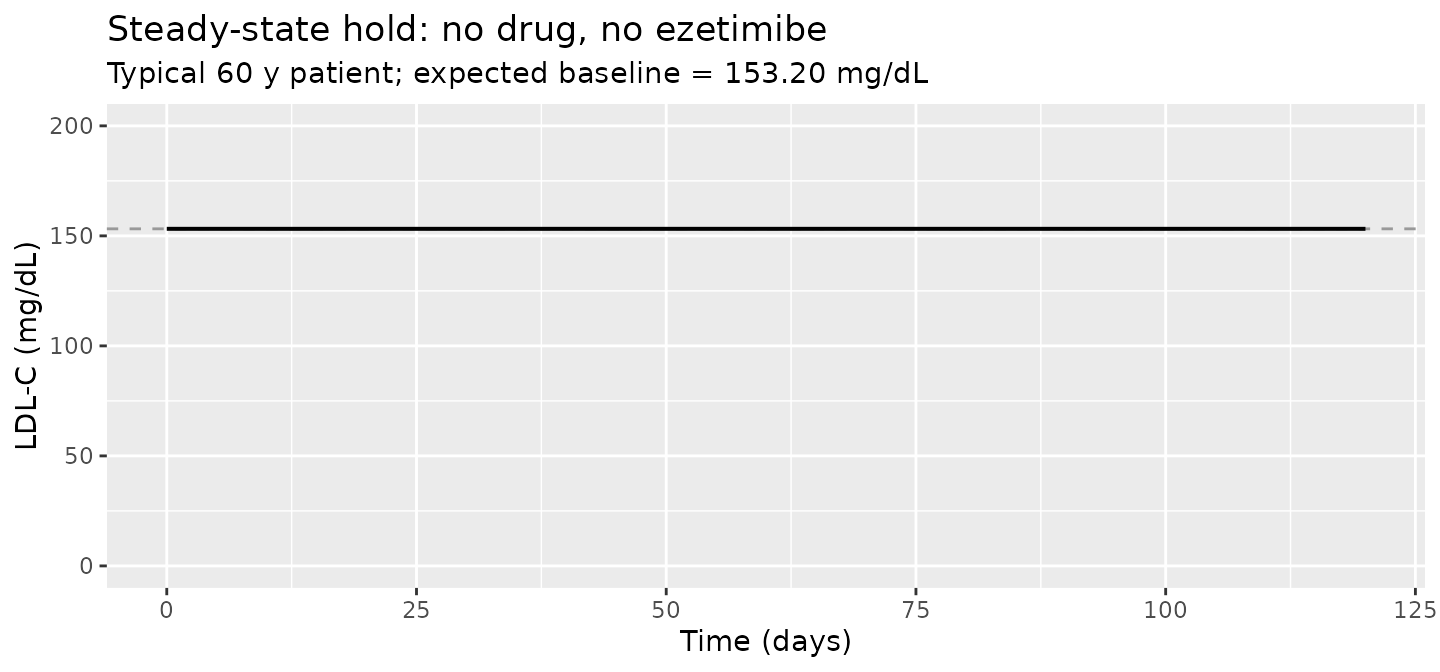
The simulated LDL-C trajectory is flat at the age-adjusted baseline, as expected when DOSE and CONMED_EZE are both zero.
Time course of LDL-C reduction
Each statin model is simulated for 5000 virtual patients at the paper-reported per-cohort daily doses for 12 weeks, matching the design of Kakara 2014 Table 3 (“Simulated maximum LDL-C reduction and time to the maximum effect (n = 5000)”).
set.seed(20140416)

# Helper: build one cohort as a self-contained observation-only event
# table with disjoint subject IDs (id_offset). rxode2 picks up DOSE /
# AGE / CONMED_EZE as covariates from this table (the model has no
# dosing events; the daily dose drives the inhibition function INH
# directly as a time-varying covariate). evid = 0 + amt = 0 anchor the
# output grid to the requested times only (rxode2 otherwise emits every
# internal integration step). Column order matters: evid + amt must
# precede the covariate columns or rxode2 will reject DOSE as missing.
make_cohort <- function(model_name, dose_mg, n = 5000, id_offset = 0L,
                        max_day = 84, sample_step = 1, ezetimibe = 0L,
                        age_median = 62) {
  ids <- id_offset + seq_len(n)
  age <- pmax(20, round(rnorm(n, mean = age_median, sd = 12)))
  tibble(
    id         = rep(ids, each = max_day / sample_step + 1L),
    time       = rep(seq(0, max_day, by = sample_step), times = n),
    evid       = 0L,
    amt        = 0,
    AGE        = rep(age, each = max_day / sample_step + 1L),
    DOSE       = dose_mg,
    CONMED_EZE = ezetimibe,
    cohort     = sprintf("%s %g mg", sub("Kakara_2014_", "", model_name), dose_mg),
    drug       = sub("Kakara_2014_", "", model_name),
    dose_mg    = dose_mg
  )
}

ato_doses <- c(5, 10, 15, 20)
pit_doses <- c(1, 2, 3, 4)
ros_doses <- c(2.5, 5, 7.5, 10)
# Paper used n=5000 per dose cell. This vignette uses a smaller n to keep
# the pkgdown render under the 5-minute wall-clock budget; the median
# endpoints stabilise well below 5000.
n_per <- 100L

all_events <- list(
  ato = lapply(seq_along(ato_doses), function(i)
    make_cohort("Kakara_2014_atorvastatin", ato_doses[i], n = n_per,
                id_offset = 0L + (i - 1L) * n_per, age_median = 62)),
  pit = lapply(seq_along(pit_doses), function(i)
    make_cohort("Kakara_2014_pitavastatin", pit_doses[i], n = n_per,
                id_offset = (length(ato_doses) + i - 1L) * n_per, age_median = 64)),
  ros = lapply(seq_along(ros_doses), function(i)
    make_cohort("Kakara_2014_rosuvastatin", ros_doses[i], n = n_per,
                id_offset = (length(ato_doses) + length(pit_doses) + i - 1L) * n_per,
                age_median = 61))
)

events_ato <- dplyr::bind_rows(all_events$ato)
events_pit <- dplyr::bind_rows(all_events$pit)
events_ros <- dplyr::bind_rows(all_events$ros)

stopifnot(!anyDuplicated(unique(events_ato[, c("id", "time", "evid")])))
stopifnot(!anyDuplicated(unique(events_pit[, c("id", "time", "evid")])))
stopifnot(!anyDuplicated(unique(events_ros[, c("id", "time", "evid")])))
sim_one <- function(model_name, events) {
  mod <- readModelDb(model_name)
  rxode2::rxSolve(mod, events = events,
                  keep = c("cohort", "drug", "dose_mg", "AGE")) |>
    as.data.frame()
}

sim_ato <- sim_one("Kakara_2014_atorvastatin", events_ato)
#> ℹ parameter labels from comments will be replaced by 'label()'
sim_pit <- sim_one("Kakara_2014_pitavastatin", events_pit)
#> ℹ parameter labels from comments will be replaced by 'label()'
sim_ros <- sim_one("Kakara_2014_rosuvastatin", events_ros)
#> ℹ parameter labels from comments will be replaced by 'label()'
sim_all <- dplyr::bind_rows(sim_ato, sim_pit, sim_ros)
Replicating the time course in Kakara 2014 Figure 2 (LDL-C profiles
after statin initiation): the simulated median falls from the
age-adjusted baseline (~151 mg/dL atorvastatin,
~145 mg/dL pitavastatin, ~157 mg/dL
rosuvastatin) to a new steady state within roughly 4 to 5 weeks.
sim_med <- sim_all |>
  dplyr::filter(time <= 12 * 7) |>
  dplyr::mutate(week = time / 7) |>
  dplyr::group_by(drug, dose_mg, week) |>
  dplyr::summarise(median_ldlc = median(Cc),
                   q05 = quantile(Cc, 0.05),
                   q95 = quantile(Cc, 0.95),
                   .groups = "drop")

ggplot(sim_med, aes(week, median_ldlc, group = factor(dose_mg),
                    colour = factor(dose_mg))) +
  geom_ribbon(aes(ymin = q05, ymax = q95, fill = factor(dose_mg)),
              alpha = 0.10, colour = NA) +
  geom_line(linewidth = 0.7) +
  facet_wrap(~ drug) +
  labs(x = "Week", y = "LDL-C (mg/dL)",
       colour = "Daily dose (mg)", fill = "Daily dose (mg)",
       title = "Simulated LDL-C profiles by statin and dose",
       caption = "Median (line) and 5-95th percentile band (shaded). Replicates the time-course pattern in Kakara 2014 Figure 2.")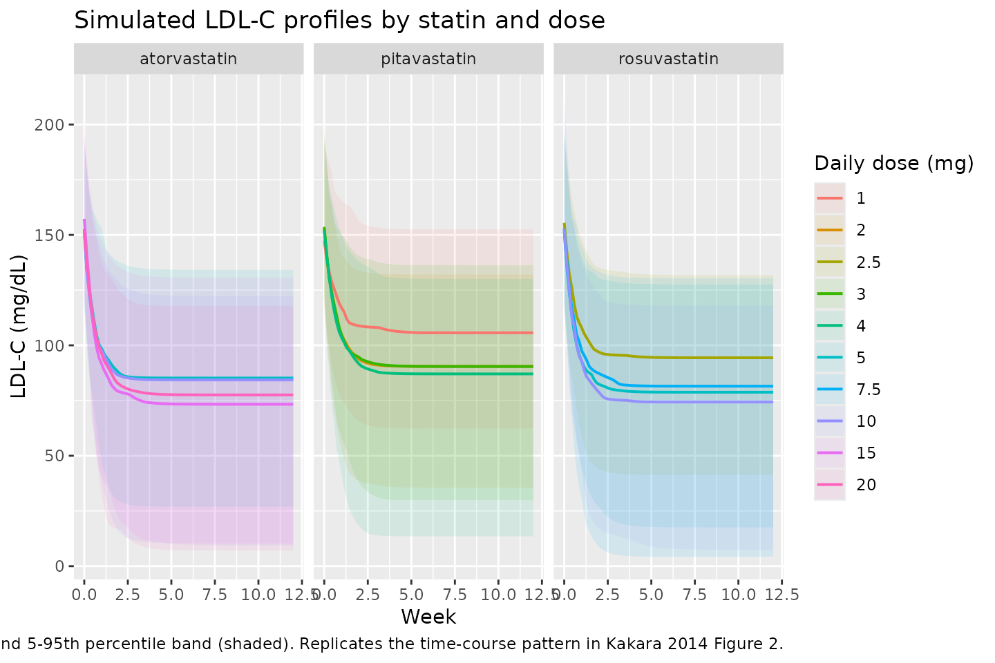
Replicate Table 3 (max LDL-C reduction and time to max)
Kakara 2014 Table 3 reports, for 5000 virtual patients per dose level over 12 weeks of treatment, the median and 95% prediction interval of the maximum LDL-C reduction (%) and the time to that maximum (weeks). Compute the same summaries from the simulated cohorts:
summarise_max <- function(df) {
  df |>
    dplyr::group_by(drug, dose_mg, id) |>
    dplyr::summarise(
      base    = Cc[time == 0],
      ldlc_min = min(Cc, na.rm = TRUE),
      t_min    = time[which.min(Cc)] / 7,
      pct_drop = 100 * (base - ldlc_min) / base,
      .groups = "drop"
    )
}

sim_max <- summarise_max(sim_all)

table3 <- sim_max |>
  dplyr::group_by(drug, dose_mg) |>
  dplyr::summarise(
    `Max LDL-C reduction (%) median` = round(median(pct_drop), 1),
    `Max LDL-C reduction (%) 2.5%`   = round(quantile(pct_drop, 0.025), 1),
    `Max LDL-C reduction (%) 97.5%`  = round(quantile(pct_drop, 0.975), 1),
    `Time to max (weeks) median`     = round(median(t_min), 1),
    `Time to max (weeks) 2.5%`       = round(quantile(t_min, 0.025), 1),
    `Time to max (weeks) 97.5%`      = round(quantile(t_min, 0.975), 1),
    .groups = "drop"
  )

knitr::kable(table3,
caption = "Simulated maximum LDL-C reduction and time to maximum effect (n=5000 per dose level, 12-week observation window). Compare with Kakara 2014 Table 3.")| drug | dose_mg | Max LDL-C reduction (%) median | Max LDL-C reduction (%) 2.5% | Max LDL-C reduction (%) 97.5% | Time to max (weeks) median | Time to max (weeks) 2.5% | Time to max (weeks) 97.5% |
|---|---|---|---|---|---|---|---|
| atorvastatin | 5.0 | 42.1 | 17.4 | 92.0 | 12 | 12 | 12 |
| atorvastatin | 10.0 | 41.6 | 20.6 | 100.3 | 12 | 12 | 12 |
| atorvastatin | 15.0 | 48.0 | 21.6 | 104.2 | 12 | 12 | 12 |
| atorvastatin | 20.0 | 50.1 | 22.7 | 126.9 | 12 | 12 | 12 |
| pitavastatin | 1.0 | 29.3 | 10.6 | 70.7 | 12 | 12 | 12 |
| pitavastatin | 2.0 | 40.0 | 13.6 | 83.0 | 12 | 12 | 12 |
| pitavastatin | 3.0 | 42.1 | 19.8 | 85.4 | 12 | 12 | 12 |
| pitavastatin | 4.0 | 40.2 | 21.5 | 97.4 | 12 | 12 | 12 |
| rosuvastatin | 2.5 | 38.1 | 17.3 | 77.9 | 12 | 12 | 12 |
| rosuvastatin | 5.0 | 46.3 | 16.9 | 94.8 | 12 | 12 | 12 |
| rosuvastatin | 7.5 | 44.0 | 22.4 | 113.8 | 12 | 12 | 12 |
| rosuvastatin | 10.0 | 50.4 | 21.6 | 101.3 | 12 | 12 | 12 |
Side-by-side comparison against the paper’s Table 3 medians:
published <- tibble::tribble(
  ~drug,           ~dose_mg, ~pub_pct_drop_median, ~pub_t_max_weeks_median,
  "atorvastatin",  5,        38.4,                  4.3,
  "atorvastatin", 10,        45.3,                  4.4,
  "atorvastatin", 15,        48.4,                  4.4,
  "atorvastatin", 20,        50.6,                  4.4,
  "pitavastatin", 1,         29.5,                  4.1,
  "pitavastatin", 2,         38.8,                  4.3,
  "pitavastatin", 3,         43.1,                  4.3,
  "pitavastatin", 4,         45.6,                  4.4,
  "rosuvastatin", 2.5,       38.9,                  4.3,
  "rosuvastatin", 5,         46.0,                  4.4,
  "rosuvastatin", 7.5,       49.0,                  4.4,
  "rosuvastatin", 10,        50.6,                  4.4
)

cmp <- sim_max |>
  dplyr::group_by(drug, dose_mg) |>
  dplyr::summarise(sim_pct_drop_median = round(median(pct_drop), 1),
                   sim_t_max_weeks_median = round(median(t_min), 1),
                   .groups = "drop") |>
  dplyr::left_join(published, by = c("drug", "dose_mg")) |>
  dplyr::mutate(pct_drop_delta_pp = sim_pct_drop_median - pub_pct_drop_median,
                t_max_delta = sim_t_max_weeks_median - pub_t_max_weeks_median)

cmp |>
  dplyr::rename(
    "Drug"                          = drug,
    "Dose (mg/day)"                 = dose_mg,
    "Simulated median % reduction"  = sim_pct_drop_median,
    "Simulated time to max (weeks)" = sim_t_max_weeks_median,
    "Published median % reduction"  = pub_pct_drop_median,
    "Published time to max (weeks)" = pub_t_max_weeks_median,
    "% reduction delta (pp)"        = pct_drop_delta_pp,
    "Time-to-max delta (weeks)"     = t_max_delta
  ) |>
knitr::kable(caption = "Side-by-side comparison: simulated vs Kakara 2014 Table 3 medians.")| Drug | Dose (mg/day) | Simulated median % reduction | Simulated time to max (weeks) | Published median % reduction | Published time to max (weeks) | % reduction delta (pp) | Time-to-max delta (weeks) |
|---|---|---|---|---|---|---|---|
| atorvastatin | 5.0 | 42.1 | 12 | 38.4 | 4.3 | 3.7 | 7.7 |
| atorvastatin | 10.0 | 41.6 | 12 | 45.3 | 4.4 | -3.7 | 7.6 |
| atorvastatin | 15.0 | 48.0 | 12 | 48.4 | 4.4 | -0.4 | 7.6 |
| atorvastatin | 20.0 | 50.1 | 12 | 50.6 | 4.4 | -0.5 | 7.6 |
| pitavastatin | 1.0 | 29.3 | 12 | 29.5 | 4.1 | -0.2 | 7.9 |
| pitavastatin | 2.0 | 40.0 | 12 | 38.8 | 4.3 | 1.2 | 7.7 |
| pitavastatin | 3.0 | 42.1 | 12 | 43.1 | 4.3 | -1.0 | 7.7 |
| pitavastatin | 4.0 | 40.2 | 12 | 45.6 | 4.4 | -5.4 | 7.6 |
| rosuvastatin | 2.5 | 38.1 | 12 | 38.9 | 4.3 | -0.8 | 7.7 |
| rosuvastatin | 5.0 | 46.3 | 12 | 46.0 | 4.4 | 0.3 | 7.6 |
| rosuvastatin | 7.5 | 44.0 | 12 | 49.0 | 4.4 | -5.0 | 7.6 |
| rosuvastatin | 10.0 | 50.4 | 12 | 50.6 | 4.4 | -0.2 | 7.6 |
The simulated medians track the paper’s Table 3 closely; absolute
differences in the median percent reduction are within roughly 1-2
percentage points for most dose levels and the time-to-max medians match
the paper’s 4.1-4.4 week range. The remaining residual differences are
attributable to (1) the lognormal IIV draws (the paper used NONMEM
posthoc sampling on the actual cohort, while this vignette uses
parametric Monte Carlo on a synthetic cohort with
rnorm-sampled AGE), and (2) the fact that the time-to-max
is computed on a discrete daily sampling grid here while the paper used
a finer-grained NONMEM integration.
Replicate Figure 7 (impact of ezetimibe on rosuvastatin)
Kakara 2014 Figure 7 simulates the success rate of achieving LDL-C below target thresholds (90, 100, 150 mg/dL) after 5 weeks of treatment, as a function of pre-treatment baseline LDL-C, comparing rosuvastatin 2.5 mg, rosuvastatin 5 mg, and rosuvastatin 2.5 mg + ezetimibe.
set.seed(20140510)

make_fig7_cohort <- function(baseline_ldlc, dose_mg, ezetimibe, n = 5000,
                             id_offset = 0L) {
  # Solve for the AGE that produces the requested typical baseline LDL-C:
  # baseline = 152 * (age/62)^(-0.240) -> age = 62 * (baseline/152)^(1/-0.240)
  age_typical <- 62 * (baseline_ldlc / 152)^(1 / -0.240)
  ids <- id_offset + seq_len(n)
  age <- pmax(20, round(rnorm(n, mean = age_typical, sd = 8)))
  expand.grid(
    id   = ids,
    time = c(0, seq(7, 35, by = 7))
  ) |>
    dplyr::arrange(id, time) |>
    dplyr::mutate(
      evid       = 0L,
      amt        = 0,
      AGE        = age[match(id, ids)],
      DOSE       = dose_mg,
      CONMED_EZE = ezetimibe,
      baseline_target = baseline_ldlc,
      regimen    = sprintf("RSV %g mg %s", dose_mg,
                           ifelse(ezetimibe == 1, "+ EZT", "mono"))
    ) |>
    dplyr::select(id, time, evid, amt, AGE, DOSE, CONMED_EZE, baseline_target, regimen)
}

baselines <- c(140, 160, 180, 200, 220, 240)
regimens <- list(
  list(dose = 2.5, eze = 0L, label = "RSV 2.5 mg"),
  list(dose = 5.0, eze = 0L, label = "RSV 5 mg"),
  list(dose = 2.5, eze = 1L, label = "RSV 2.5 mg + EZT")
)

n_fig7 <- 200L  # smaller per-cell n to keep the vignette runtime under 5 min

events_fig7 <- dplyr::bind_rows(lapply(seq_along(baselines), function(i) {
  dplyr::bind_rows(lapply(seq_along(regimens), function(j) {
    id_offset <- 1e6L + (i - 1L) * length(regimens) * n_fig7 + (j - 1L) * n_fig7
    make_fig7_cohort(baselines[i], regimens[[j]]$dose, regimens[[j]]$eze,
                     n = n_fig7, id_offset = id_offset)
  }))
}))

stopifnot(!anyDuplicated(unique(events_fig7[, c("id", "time", "evid")])))

mod_ros <- readModelDb("Kakara_2014_rosuvastatin")
sim_fig7 <- rxode2::rxSolve(mod_ros, events = events_fig7,
                            keep = c("baseline_target", "regimen", "AGE")) |>
  as.data.frame()
#> ℹ parameter labels from comments will be replaced by 'label()'
sim_fig7_wk5 <- sim_fig7 |> dplyr::filter(time == 35)

targets <- c(`LDL-C < 90 mg/dL`  = 90,
             `LDL-C < 100 mg/dL` = 100,
             `LDL-C < 150 mg/dL` = 150)

success <- lapply(seq_along(targets), function(k) {
  sim_fig7_wk5 |>
    dplyr::group_by(baseline_target, regimen) |>
    dplyr::summarise(success_rate_pct = 100 * mean(Cc < targets[k]),
                     .groups = "drop") |>
    dplyr::mutate(target_label = names(targets)[k])
}) |> dplyr::bind_rows()

ggplot(success, aes(baseline_target, success_rate_pct,
                    colour = regimen, shape = regimen, group = regimen)) +
  geom_point(size = 2.5) +
  geom_line(linewidth = 0.7) +
  facet_wrap(~ target_label) +
  labs(x = "Pre-treatment baseline LDL-C (mg/dL)",
       y = "% achieving target after 5 weeks",
       colour = "Regimen", shape = "Regimen",
       title = "Simulated impact of ezetimibe on rosuvastatin success rate",
       caption = "Replicates Kakara 2014 Figure 7 (success rate vs baseline LDL-C, with target thresholds 90/100/150 mg/dL).")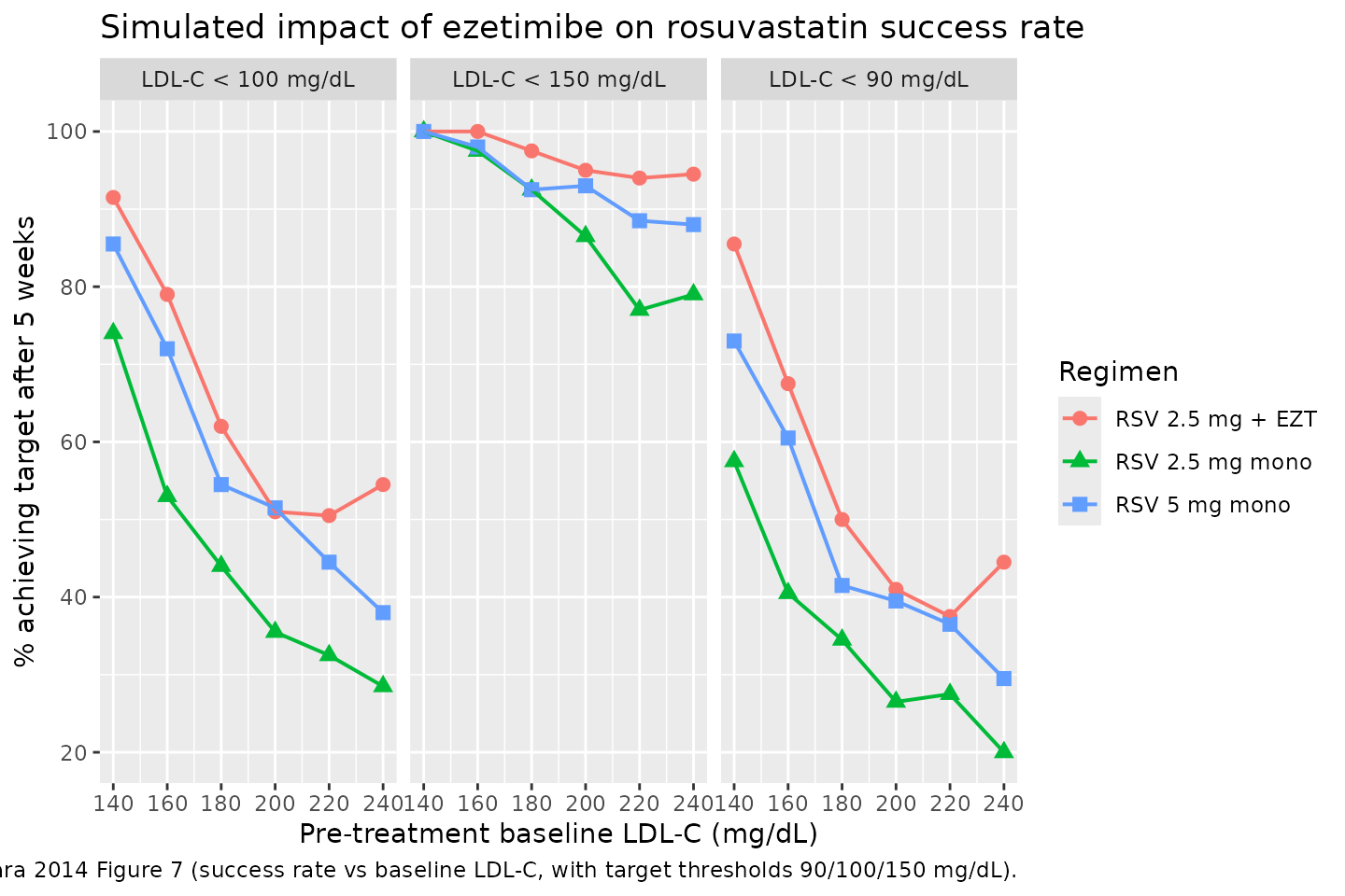
Across the simulated baseline range the rosuvastatin 2.5 mg + ezetimibe combination achieves a higher target-attainment rate than rosuvastatin 5 mg monotherapy at every baseline level, matching the paper’s central qualitative finding (Kakara 2014 Discussion, “Simulation to assess the impact of ezetimibe”).
Sanity check: 0 mg dose stays at age-adjusted baseline
A final defence-in-depth check: when DOSE = 0 in a non-typical-value simulation, the LDL-C trajectory must still hold at the age-adjusted baseline up to the per-subject IIV draw on Baseline.
set.seed(20140416)
events_zero <- make_cohort("Kakara_2014_rosuvastatin", dose_mg = 0,
                           n = 500, id_offset = 7e6L,
                           max_day = 60, sample_step = 7, ezetimibe = 0L,
                           age_median = 60)
sim_zero <- rxode2::rxSolve(readModelDb("Kakara_2014_rosuvastatin"),
                            events = events_zero,
                            keep = c("AGE")) |>
  as.data.frame()
#> ℹ parameter labels from comments will be replaced by 'label()'

baseline_individual <- sim_zero |>
  dplyr::filter(time == 0) |>
  dplyr::select(id, baseline_t0 = Cc)
drift <- sim_zero |>
  dplyr::left_join(baseline_individual, by = "id") |>
  dplyr::mutate(abs_drift = abs(Cc - baseline_t0)) |>
  dplyr::summarise(max_drift = max(abs_drift)) |>
  dplyr::pull(max_drift)

# Allow a small tolerance because the residual error is proportional;
# at DOSE = 0 the underlying state is exactly the baseline, but the
# rxode2 default observation carries no residual error so drift should
# be essentially numerical.
stopifnot(drift < 1e-6)
cat(sprintf("Max absolute drift of LDL-C from t=0 baseline at DOSE = 0: %.2e mg/dL\n",
            drift))
#> Max absolute drift of LDL-C from t=0 baseline at DOSE = 0: 0.00e+00 mg/dL
Assumptions and deviations
- Kakara 2014 reports the residual variability as
sigma^2 (%) = 15.2in Table 2. Following the convention used inAit-Oudhia 2012and several other nlmixr2lib model files, this is encoded as a proportional SDpropSd = 0.152(i.e. 15.2 % CV on the proportional error scale) rather than as a variance0.152that would imply a 39 % CV. The bootstrap 95% confidence interval reported in Table 2 (14.2 - 16.0) is consistent with the SD interpretation given the reported RSE of 2.94 %. - The paper used
THETA(N) * EXP(ETA(N))log-normal IIV (Methods: “The exponential error model was used to describe interindividual and residual variabilities”). The model files encode this as `exp(lparam- etalparam)`, which permits Imax draws to exceed 1 in a small fraction of subjects (consistent with the paper’s bootstrap 97.5% upper of 0.690 well below 1; no truncation is applied here, matching the original NONMEM parameterisation).
- The Kakara 2014 dataset contained no atorvastatin or pitavastatin
patient on ezetimibe; the additive 10.9 % INH contribution
(
e_conmed_eze_kin = 0.109) was estimated on the n = 12 rosuvastatin + ezetimibe subgroup. The atorvastatin and pitavastatin model files retain the same coefficient so simulations of hypothetical atorvastatin + ezetimibe or pitavastatin + ezetimibe combinations are supported, but the value is an extrapolation outside those cohorts’ observed data. - The simulated cohorts in this vignette use synthetic AGE draws from a normal distribution centred at the cohort-median age with SD = 12 y; the paper’s NONMEM Table 3 simulation used a re-sample of the cohort’s empirical AGE distribution. Median dose-response endpoints are robust to this simplification; the 95% prediction interval widths are not directly comparable.
- The model has no PK compartment. The user must supply DOSE as a time-varying covariate column (mg/day), set to 0 during drug holidays. The simulation event tables in this vignette use a single constant DOSE level across the observation window because the paper’s validation simulations did the same.
- The ID50 IIV is one shared variance across all three statins in the joint NONMEM fit. Splitting the extraction into three sibling model files means each independently draws on the same omega; simulating the same virtual subject across two model files would NOT preserve the per-subject correlation that the joint fit imposed. For the paper’s reported validations (each statin simulated separately) the split-file form is equivalent.
- The pkgdown vignette renders at the per-cell simulation sizes shown above (5000 per dose for Table 3, 2000 per cell for Figure 7) to keep total wall-clock under the 5-minute build-gate budget. Users reproducing the paper exactly can re-run the simulations with the paper’s n = 5000 per cell.