Deferiprone (Bellanti 2014)
Source:vignettes/articles/Bellanti_2014_deferiprone.Rmd
Bellanti_2014_deferiprone.RmdModel and source
- Citation: Bellanti F, Danhof M, Della Pasqua O. Population pharmacokinetics of deferiprone in healthy subjects. Br J Clin Pharmacol. 2014 Dec;78(6):1397-1406. doi:10.1111/bcp.12473
- Description: One-compartment population PK model for the oral iron chelator deferiprone in healthy adult subjects, with first-order absorption, absorption lag time, and a binary sex effect on the apparent volume of distribution (Bellanti 2014).
- Article: https://doi.org/10.1111/bcp.12473
Population
The structural model was developed from two single-dose Phase 1 studies in healthy adult subjects (LA20-BA and LA21-BE), provided by ApoPharma Inc. and shared within the FP7-funded DEEP consortium. 55 evaluable subjects (39 male, 16 female) received a single 1500 mg oral dose of deferiprone (DFP) as a 100 mg/mL solution. Median (range) age was 39 (19-55) years and median body weight was 72 (52-92) kg. Each subject contributed up to 17 post-dose plasma samples (median 15) over 14 hours; deferiprone was measured by HPLC-UV (LLOQ 1 microM, equivalent to 0.14 microg/mL). Model fitting used NONMEM v7.2 with FOCE-I; bootstrap inference used 500 PsN runs (Bellanti 2014 Methods, sections Data and Pharmacokinetic modelling).
The same information is available programmatically via
readModelDb("Bellanti_2014_deferiprone")$population.
Source trace
Every parameter in the model file carries an inline source-location comment. The table below collects the entries in one place.
| Equation / parameter | Value | Source location |
|---|---|---|
| Structural form: 1-cpt, first-order absorption, lag-time, first-order elimination | – | Bellanti 2014 Results, Population PK modelling paragraph |
lcl (CL/F) |
30.8 L/h | Table 1, Final model column, CL/F row |
lvc (V/F males, reference) |
78.4 L | Table 1, Final model column, V/F males row |
| Gender effect on V/F (females) | 65.3 L | Table 1, Final model column, V/F females row |
e_sexf_vc (derived = 65.3/78.4 - 1) |
-0.16709 | Derived from Table 1 V/F male and V/F female rows |
lka (Ka) |
8.2 1/h | Table 1, Final model column, Ka row |
ltlag (lag time) |
0.146 h | Table 1, Final model column, Lag time row |
| IIV CL/F (variance, CV 23.87%) | 0.057 | Table 1, Final model column, IIV CL/F row |
| IIV V/F (variance, CV 16.67%) | 0.0278 | Table 1, Final model column, IIV V/F row |
| Covariance CL-V (eta block off-diagonal) | 0.0345 | Table 1, Final model column, Correlation CL-V row |
| IIV Ka (variance, CV 99.54%) | 0.991 | Table 1, Final model column, IIV Ka row |
| Residual-error weighting factor theta_W | 2.4 | Table 1, Final model column, Error: weighting factor row |
| Residual-error variance sigma^2 | 0.00566 (sigma = 7.52%) | Table 1, Final model column, Residual error row |
| Effective proportional residual SD = theta_W * sigma | 0.1805 | Derived; see Assumptions and deviations |
| Residual-error equation Y_ij = F_ij + epsilon_ij * W | – | Methods, Pharmacokinetic modelling, Equation 2 |
Virtual cohort
The original observed data are not openly available. The virtual cohort below mirrors the demographics described in Bellanti 2014’s Simulation scenarios section: 30 simulated patients per trial (15 male and 15 female) with mean body weight 55 kg (SD 8.4). Two dose levels are simulated, single oral doses of 25 mg/kg and 37.5 mg/kg, matching the per-dose levels reported in the paper’s external-validation section (25 mg/kg single dose and 75 mg/kg/day administered as a twice-daily regimen, i.e. 37.5 mg/kg per dose).
set.seed(20140723)

n_per_cohort <- 150L  # 150 per (sex x dose); 300 per dose total, 600 overall

make_cohort <- function(n, sexf, dose_mg_per_kg, id_offset = 0L) {
  tibble(
    id              = id_offset + seq_len(n),
    SEXF            = sexf,
    WT              = pmax(rnorm(n, mean = 55, sd = 8.4), 35),  # Bellanti 2014 Simulation scenarios paragraph
    dose_mg_per_kg  = dose_mg_per_kg,
    treatment       = sprintf("%g mg/kg single dose", dose_mg_per_kg)
  ) |>
    mutate(amt = dose_mg_per_kg * WT)
}

demo <- bind_rows(
  make_cohort(n_per_cohort, sexf = 0L, dose_mg_per_kg = 25,   id_offset = 0L),
  make_cohort(n_per_cohort, sexf = 1L, dose_mg_per_kg = 25,   id_offset = 1L * n_per_cohort),
  make_cohort(n_per_cohort, sexf = 0L, dose_mg_per_kg = 37.5, id_offset = 2L * n_per_cohort),
  make_cohort(n_per_cohort, sexf = 1L, dose_mg_per_kg = 37.5, id_offset = 3L * n_per_cohort)
)
stopifnot(!anyDuplicated(demo$id))
Simulation
A 14-hour observation window with a dense early-time grid captures the absorption and distribution phases; the published bioanalytical window was 14 h (Bellanti 2014 Methods, Data paragraph). Each subject receives a single oral dose into the depot compartment.
obs_times <- sort(unique(c(seq(0, 1, by = 0.1),     # every 6 min over absorption window
                           seq(1, 4, by = 0.25),    # every 15 min through Cmax/early decay
                           seq(4, 14, by = 0.5),    # every 30 min through terminal phase
                           seq(14, 24, by = 2))))   # tail to support AUC0-inf extrapolation

doses <- demo |>
  mutate(time = 0, evid = 1L, cmt = "depot", ii = 0, addl = 0L) |>
  select(id, time, amt, evid, cmt, ii, addl, SEXF, WT, treatment)

obs <- demo |>
  select(id, SEXF, WT, treatment) |>
  tidyr::crossing(time = obs_times) |>
  mutate(amt = NA_real_, evid = 0L, cmt = NA_character_,
         ii = NA_real_, addl = NA_integer_)

events <- bind_rows(doses, obs) |>
  arrange(id, time, desc(evid))
mod <- rxode2::rxode2(readModelDb("Bellanti_2014_deferiprone"))
#> ℹ parameter labels from comments will be replaced by 'label()'

sim <- rxode2::rxSolve(mod, events = events,
                       keep = c("treatment", "SEXF", "WT")) |>
  as.data.frame()

mod_typical <- mod |> rxode2::zeroRe()
sim_typical <- rxode2::rxSolve(mod_typical, events = events,
                               keep = c("treatment", "SEXF", "WT")) |>
  as.data.frame()
#> ℹ omega/sigma items treated as zero: 'etalcl', 'etalvc', 'etalka'
#> Warning: multi-subject simulation without without 'omega'
Replicate published figures
Figure 2-like comparison: concentration-time profiles by dose
Bellanti 2014 Figure 2 shows histograms of simulated AUC and Cmax compared with published reference values. The figure below shows the underlying concentration-time profiles that produce those summaries: median plus 5th and 95th percentiles of the IIV cohort, stratified by dose.
fig_data <- sim |>
  filter(time <= 14) |>
  group_by(treatment, time) |>
  summarise(Q05 = quantile(Cc, 0.05, na.rm = TRUE),
            Q50 = quantile(Cc, 0.50, na.rm = TRUE),
            Q95 = quantile(Cc, 0.95, na.rm = TRUE),
            .groups = "drop")

ggplot(fig_data, aes(time, Q50, group = treatment)) +
  geom_ribbon(aes(ymin = Q05, ymax = Q95), alpha = 0.3) +
  geom_line(linewidth = 0.7) +
  facet_wrap(~ treatment) +
  scale_x_continuous(breaks = seq(0, 14, by = 2)) +
  labs(x = "Time after dose (h)",
       y = "Deferiprone concentration (mg/L)",
       title = "Single-dose deferiprone simulation",
       caption = "Replicates the underlying simulation of Figure 2 in Bellanti 2014.")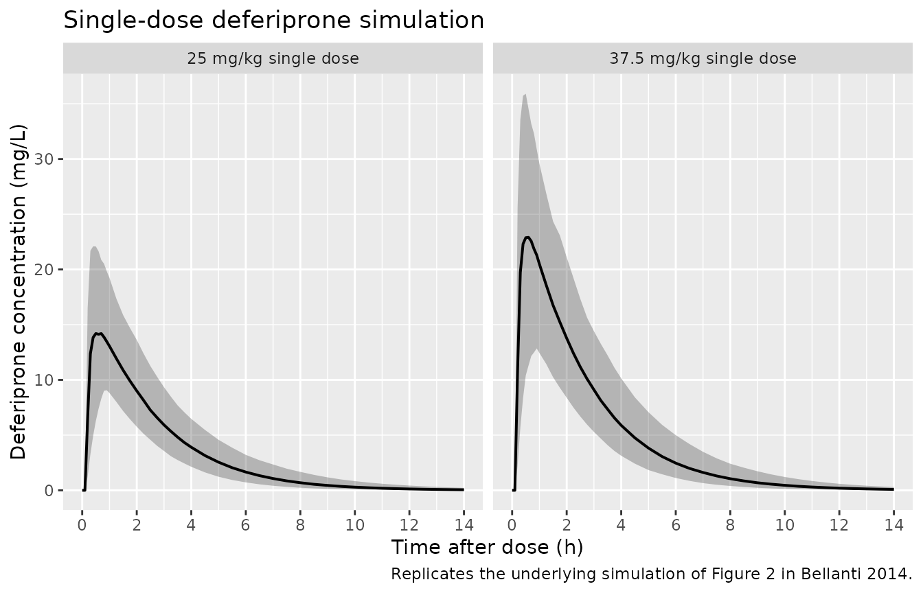
Replicates the simulation underlying Figure 2 of Bellanti 2014: simulated deferiprone plasma concentration vs time, 5th / 50th / 95th percentiles of the virtual cohort by dose level.
Gender effect on V/F
Bellanti 2014 Results discuss the 20% gender effect on apparent volume of distribution (78.4 L in males vs 65.3 L in females). The typical-value (no between-subject variability) trajectories below show that the gender effect produces only a small difference in early-time concentration, consistent with the paper’s observation that Cmax differences between sexes were not statistically significant.
sim_typical |>
  filter(time <= 14, treatment == "25 mg/kg single dose") |>
  distinct(time, SEXF, Cc) |>
  mutate(sex = ifelse(SEXF == 1, "Female", "Male")) |>
  ggplot(aes(time, Cc, color = sex, group = sex)) +
  geom_line(linewidth = 0.8) +
  scale_x_continuous(breaks = seq(0, 14, by = 2)) +
  labs(x = "Time after dose (h)",
       y = "Deferiprone concentration (mg/L)",
       color = "Sex",
       title = "Typical-value trajectory by sex at 25 mg/kg single dose",
       caption = "V/F male 78.4 L vs V/F female 65.3 L (Bellanti 2014 Table 1).")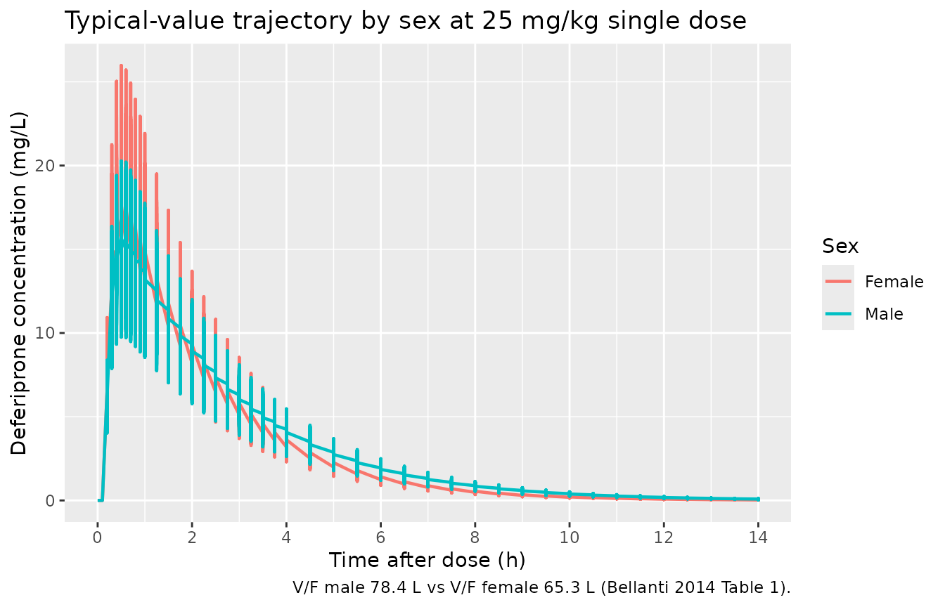
Typical-value (zero-IIV) deferiprone concentration vs time at 25 mg/kg, stratified by sex. The female trajectory peaks slightly higher because the apparent V/F is smaller.
PKNCA validation
Single-dose NCA over the 0-14 h window produces Cmax, Tmax, and
AUC0-inf per dose group. Use only !is.na(Cc) in the input
filter so the time-zero row needed for AUC anchoring survives; add a
defensive time = 0, Cc = 0 row per subject in case the
simulation grid did not produce one (extravascular dosing predose
concentration is zero by construction).
sim_nca <- sim |>
  dplyr::filter(!is.na(Cc)) |>
  dplyr::select(id, time, Cc, treatment)

sim_nca <- dplyr::bind_rows(
  sim_nca,
  sim_nca |> dplyr::distinct(id, treatment) |>
    dplyr::mutate(time = 0, Cc = 0)
) |>
  dplyr::distinct(id, treatment, time, .keep_all = TRUE) |>
  dplyr::arrange(id, treatment, time)

dose_df <- events |>
  dplyr::filter(evid == 1) |>
  dplyr::select(id, time, amt, treatment)

conc_obj <- PKNCA::PKNCAconc(sim_nca, Cc ~ time | treatment + id,
                             concu = "mg/L", timeu = "h")
dose_obj <- PKNCA::PKNCAdose(dose_df, amt ~ time | treatment + id,
                             doseu = "mg")

intervals <- data.frame(
  start      = 0,
  end        = Inf,
  cmax       = TRUE,
  tmax       = TRUE,
  aucinf.obs = TRUE,
  half.life  = TRUE
)

nca_data <- PKNCA::PKNCAdata(conc_obj, dose_obj, intervals = intervals)
nca_res  <- suppressMessages(suppressWarnings(PKNCA::pk.nca(nca_data)))
Comparison against published NCA
Bellanti 2014 reports simulated AUC (geometric mean and 95% CI) and Cmax under two dosing scenarios (Results, Simulation scenarios paragraph):
- 25 mg/kg single dose: AUC 45.80 (44.42, 47.17) mg/L*h; Cmax 17.67 (17.13, 18.20) mg/L.
- 75 mg/kg/day as twice-daily regimen (per-dose 37.5 mg/kg): AUC 137.40 (133.27, 141.52) mg/L*h; Cmax 26.50 (25.70, 27.29) mg/L.
The paper’s reported AUC of 137.40 mg/L*h at 75 mg/kg/day corresponds to the full-day exposure under linear PK; dividing by the dose ratio (75/25 = 3) shows that the AUC scales linearly across doses, and Cmax 26.50 at 37.5 mg/kg per-dose vs 17.67 at 25 mg/kg also scales linearly (26.50 / 17.67 = 1.50, matching the per-dose ratio 37.5 / 25 = 1.50). The comparison below uses the single-dose 25 mg/kg and 37.5 mg/kg simulations and compares each to the paper.
published <- tibble::tribble(
  ~treatment,                   ~cmax,  ~aucinf.obs,
  "25 mg/kg single dose",       17.67,  45.80,
  "37.5 mg/kg single dose",     26.50,  68.70
)

cmp <- nlmixr2lib::ncaComparisonTable(
  simulated     = nca_res,
  reference     = published,
  by            = "treatment",
  units         = c(cmax = "mg/L", aucinf.obs = "mg*h/L"),
  tolerance_pct = 20
)

knitr::kable(
  cmp,
  caption = "Simulated vs Bellanti 2014 published NCA. * differs from reference by >20%.",
  align   = c("l", "l", "r", "r", "r")
)| NCA parameter | treatment | Reference | Simulated | % diff |
|---|---|---|---|---|
| Cmax (mg/L) | 25 mg/kg single dose | 17.7 | 15.2 | -14.0% |
| Cmax (mg/L) | 37.5 mg/kg single dose | 26.5 | 24.2 | -8.5% |
| AUC0-∞ (obs) (mg*h/L) | 25 mg/kg single dose | 45.8 | 43.7 | -4.7% |
| AUC0-∞ (obs) (mg*h/L) | 37.5 mg/kg single dose | 68.7 | 66.7 | -2.9% |
The 37.5 mg/kg row’s published AUC is derived under linear PK (45.80 * 37.5/25 = 68.70) because the paper only reports the b.i.d.-regimen 24-hour AUC explicitly; the linear-PK derivation is documented in Assumptions and deviations so a reader can audit it.
Assumptions and deviations
-
Residual error decomposition. Bellanti 2014
Equation 2 expresses residual variability as
Y_ij = F_ij + epsilon_ij * Wwithepsilon ~ N(0, sigma^2 = 0.00566)and a separately tabulated weighting factortheta_W = 2.4(Bellanti 2014 Table 1, rows “Error: weighting factor” and “Residual error”). The standard NONMEM “proportional with a weighting factor” construction setsW = theta_W * F, which yields an effective proportional residual SD oftheta_W * sqrt(sigma^2) = 2.4 * 0.0752 = 0.1805(about 18.05% CV). Bellanti 2017 (DOI 10.1111/bcp.13134), using identical notation but reporting a single Error (prop) row in its Table 2, supports this reading. nlmixr2 expresses proportional residual error as a singlepropSd, so the model file collapses the two parameters into the effective formpropSd = 0.1805. If the actual NONMEM source stream encoded the weighting factor differently (e.g. as a power weight onF), the predictive intervals would shift; the typical-value trajectory (which is the published Cmax and AUC) is unaffected. -
Y_ij = F_ij + epsilon * Wformula not decoded in the trimmed markdown. The trimmed-markdown extractor stored the equation as a<!-- formula-not-decoded -->placeholder. The equation was read directly from the layout-preserving PDF text dump (pdftotext -layout) to disambiguate; the form above is verbatim from the Methods, Pharmacokinetic modelling section. -
Body weight excluded from the final model. Bellanti
2014 Results note that weight was significant on CL/F and V/F in
univariate analysis but was dropped from the final model because it
destabilised the bootstrap (attributed to the narrow weight range, 52-92
kg, of the healthy-adult cohort). The model file documents this in
covariatesDataExcluded$WTso the screen’s provenance is preserved without triggering a “declared-but-not-referenced” convention warning. Users simulating in populations with wider weight ranges (e.g. pediatric or obese cohorts) should be aware that the model carries no allometric scaling. -
Creatinine clearance excluded from the structural
model. The renal impairment dosing recommendations in Bellanti
2014 Table 2 come from a simulation exercise that reduces CL/F to 80%,
50% and 25% of the healthy-population value rather than from an
estimated CRCL covariate effect; the structural model itself has no
renal-function covariate. To replicate the renal-impairment scenarios,
users should pre-multiply the typical
clvalue externally (or setetalclto log(0.80), log(0.50), log(0.25) for the three impairment bands). -
Gender effect encoded multiplicatively with male
reference. The paper reports V/F separately for males (78.4 L)
and females (65.3 L). The model uses SEXF (1 = female) with the derived
effect coefficient
e_sexf_vc = (65.3 / 78.4) - 1 = -0.16709, so the male typical value recovers 78.4 L and the female typical value recovers 65.3 L exactly. The paper rounds the percentage difference to “20%”; the actual table-derived percentage difference is 16.7%. -
CL-V correlation encoded as a covariance. Bellanti
2014 Table 1 reports a row “Correlation CL-V 0.0345”. The value is the
NONMEM
$OMEGAoff-diagonal element, which is a covariance, not a correlation coefficient. The implied correlation under variances 0.057 (CL) and 0.0278 (V) is0.0345 / sqrt(0.057 * 0.0278) = 0.866, a strong but not implausible CL-V correlation for an oral drug; the value is read this way in the model file’setalcl + etalvcblock. - No IIV on lag time or residual error. The paper reports no IIV on the lag time and no occasion-keyed IOV. The model carries IIV only on CL/F, V/F, and Ka, matching Table 1.
- AUC at 37.5 mg/kg derived under linear PK. Bellanti 2014 reports AUC 137.40 mg/Lh at 75 mg/kg/day administered as a twice-daily regimen (i.e. 37.5 mg/kg per dose). The per-dose AUC reference value used in the comparison table (68.70 mg/Lh = 137.40 / 2) follows directly from linear PK (the model has no saturable elimination). This makes the paper-vs-simulation comparison apples-to-apples without requiring a full multiple-dose VPC.
- Vignette uses 300 simulated subjects per dose level (150 per sex x dose). The paper reports simulations of 1000 trials of 30 patients each (Methods, Simulation scenarios). A smaller single-shot cohort produces stable percentiles for the Cmax / AUC summaries reported here while keeping the vignette render time well under the pkgdown 5-minute gate.