Model and source
mod <- readModelDb("Chen_2024_nadroparin")
ui  <- rxode2::rxode(mod)
#> ℹ parameter labels from comments will be replaced by 'label()'- Citation: Chen Y, Lan J, Zhu L, Dong M, Wang Y, Li Z. Is the current therapeutic dosage of nadroparin adequate for neonates and infants under 8 months with thromboembolic disease? a population pharmacokinetic study from a national children’s medical center. Front Pharmacol. 2024 Jan 31;15:1331673. doi:10.3389/fphar.2024.1331673
- Article: https://doi.org/10.3389/fphar.2024.1331673
- PubMed Central: https://www.ncbi.nlm.nih.gov/pmc/articles/PMC10864485/
Chen 2024 is the first population pharmacokinetic analysis of nadroparin, a low-molecular-weight heparin, in preterm and term neonates and infants under 8 months of age. The model is fitted to plasma anti-Xa activity rather than to a nadroparin concentration, so clearance and volume are apparent anti-Xa parameters (CL/F, Vd/F) expressed in L/h and L, and the observation is in IU/mL.
The clinical question the paper asks is whether the locally used therapeutic dose of 150-200 IU/kg every 12 h is adequate to reach the 0.5-1 IU/mL anti-Xa target in this population. Its answer – that it is not, and that higher doses would be required – is the result this vignette reproduces.
Population
The model was developed from a retrospective single-centre chart review at the Children’s Hospital of Fudan University (National Children’s Medical Center, Shanghai) covering July 2021 to December 2023. Of 51 enrolled patients, 11 were excluded because every one of their samples was below the 0.1 IU/mL limit of quantification, leaving 40 patients contributing 56 anti-Xa samples (Chen 2024 Table 1).
The cohort spans a wide maturational range: gestational age at birth 25.0-41.3 weeks (median 36.8), postnatal age 3-224 days (median 40), postmenstrual age 30.7-69.0 weeks (median 40.4), and body weight 1.2-9.3 kg (median 3.1). Renal function, the model’s only retained covariate, spans Schwartz creatinine clearance 5.3-314.7 mL/min/1.73 m^2 (median 51.1, mean 73.8, SD 62.8). Sex was 23 boys / 17 girls. Twenty-three patients had venous thrombosis and 17 arterial thrombosis. All patients received nadroparin (Fraxiparine) 150-200 IU/kg subcutaneously every 12 h per the local protocol.
Two features of the sampling design matter for interpreting the model. Essentially all samples were 4 h post-dose peak samples (Chen 2024 Methods “Blood sampling and anti-Xa determination”; the Discussion states explicitly that all samples obtained in the centre were peak concentrations), so the absorption and terminal phases are only weakly informed by the data. And samples below the limit of quantification were discarded rather than modelled.
The same information is available programmatically:
str(mod()$population, max.level = 1)
#> List of 15
#>  $ species       : chr "human"
#>  $ n_subjects    : int 40
#>  $ n_studies     : int 1
#>  $ n_observations: chr "56 anti-Xa samples from 40 patients (Chen 2024 Table 1). 51 patients were enrolled; 11 were excluded because ev"| __truncated__
#>  $ age_range     : chr "postnatal age 3-224 days (median 40 days); postmenstrual age 30.7-69.0 weeks (median 40.4 weeks); gestational a"| __truncated__
#>  $ age_median    : chr "postnatal age 40 days (postmenstrual age 40.4 weeks)"
#>  $ weight_range  : chr "1.2-9.3 kg"
#>  $ weight_median : chr "3.1 kg"
#>  $ sex_female_pct: num 42.5
#>  $ race_ethnicity: chr "Chinese (single centre in Shanghai, China; race and ethnicity are not tabulated in the paper)"
#>  $ disease_state : chr "Preterm or term neonates and infants under 8 months of age with suspected or diagnosed arterial or venous throm"| __truncated__
#>  $ dose_range    : chr "Nadroparin (Fraxiparine) 150-200 IU/kg subcutaneously every 12 h per the local treatment protocol"
#>  $ regions       : chr "China (Children's Hospital of Fudan University, National Children's Medical Center, Shanghai; single centre)"
#>  $ renal_function: chr "Schwartz creatinine clearance 5.3-314.7 mL/min/1.73 m^2 (median 51.1, mean 73.8, SD 62.8)"
#>  $ notes         : chr "Retrospective single-centre chart review of patients treated between July 2021 and December 2023 (Chen 2024 Met"| __truncated__
Source trace
Each ini() entry in
inst/modeldb/specificDrugs/Chen_2024_nadroparin.R carries
an in-file comment naming its source. They are collected here.
| Equation / parameter | Value | Source location |
|---|---|---|
lka (ka) |
0.495 1/h | Table 2, structural model (RSE 16.4%; bootstrap median 0.495, 95% CI 0.073-1.09) |
lcl (CL/F) |
0.211 L/h | Table 2, structural model (RSE 9.4%; bootstrap median 0.207, 95% CI 0.063-0.259) |
lvc (Vd/F) |
1.55 L | Table 2, structural model (RSE 13.7%; bootstrap median 1.51, 95% CI 0.02-2.79) |
e_crcl_cl |
0.238 | Table 2, covariate model row CL/F_CLCR (RSE 29.2%;
bootstrap median 0.235, 95% CI 0.056-0.381) |
| CRCL normalising median | 51.1 mL/min/1.73 m^2 | Table 1, CLCR median (supplies Cov_median of equation
(5)) |
etalcl |
0.0678689 | Table 2, IIV on CL/F = 26.5% CV; equation (1) is exponential IIV and
the Table 2 footnote defines CV as the CV of the parameter values, so
omega^2 = log(1 + 0.265^2)
|
no eta on lvc or lka
|
n/a | Results “Population PK modeling”: “The variance for volume distribution and the absorption rate constant were fixed to zero, as they approached zero during the model-building process.” |
propSd |
0.355 | Table 2, proportional residual error 35.5% CV (RSE 10.0%; bootstrap median 34.6, 95% CI 27.2-41.5) |
IIV model P_i = P_p * exp(eta_i)
|
n/a | Equation (1), Methods “Model development” |
| Residual model | n/a | Equation (2) writes the general form
OBS = IPRED * exp(eps1) + eps2; Results state the final
model is proportional and Table 2 reports only a proportional term |
Covariate model
P_i = P_p * (Cov_i / Cov_median)^theta
|
n/a | Equation (5), Methods “Model development” |
d/dt(depot), d/dt(central)
|
n/a | Results “Population PK modeling”: one-compartment model with first-order absorption from a subcutaneous compartment and first-order elimination from the central compartment |
Cc <- central / vc / 1000 |
n/a | Unit reconciliation: amounts in IU and vc in L give
IU/L; the anti-Xa assay and the 0.5-1 IU/mL target are in IU/mL (Methods
“Blood sampling and anti-Xa determination”) |
Two equations from the Methods are deliberately
absent from the model file because they were tested but
not retained in the final model: the allometric weight term of equation
(3) and the sigmoid Emax postmenstrual-age maturation function of
equation (4). Both are documented under
covariatesDataExcluded.
Structural verification
Before simulating, three deterministic checks confirm the packaged model reproduces the published parameterisation exactly.
CL0 <- 0.211; V <- 1.55; KA <- 0.495; THETA <- 0.238; CRCL_REF <- 51.1
WT_MED <- 3.1  # Chen 2024 Table 1 median body weight

# (1) At the cohort median CRCL the covariate factor is 1, so CL/F = 0.211 L/h.
cl_at_median <- CL0 * (CRCL_REF / CRCL_REF)^THETA
stopifnot(isTRUE(all.equal(cl_at_median, 0.211, tolerance = 1e-12)))

# (2) The Discussion independently reports a weight-normalised clearance of
#     0.068 L/h/kg. That number is NOT in Table 2, so it is a genuine external
#     check -- and it confirms that 0.211 L/h is an absolute typical value for
#     this cohort rather than a 70 kg-standardised CLstd (which would give
#     0.211 * (3.1/70)^0.75 = 0.020 L/h, three-fold too small).
cl_per_kg <- cl_at_median / WT_MED
stopifnot(round(cl_per_kg, 3) == 0.068)

# (3) Covariate factor across the observed CRCL range (Table 1: 5.3-314.7).
cov_factor <- (c(5.3, 51.1, 314.7) / CRCL_REF)^THETA

tibble::tibble(
  Check = c("CL/F at median CRCL (L/h)", "CL/F per kg at median WT (L/h/kg)",
            "Covariate factor at CRCL 5.3", "Covariate factor at CRCL 314.7"),
  Model = c(cl_at_median, cl_per_kg, cov_factor[1], cov_factor[3]),
  Published = c("0.211 (Table 2)", "0.068 (Discussion)", "-", "-")
) |>
knitr::kable(digits = 4, caption = "Deterministic structural checks against Chen 2024.")| Check | Model | Published |
|---|---|---|
| CL/F at median CRCL (L/h) | 0.2110 | 0.211 (Table 2) |
| CL/F per kg at median WT (L/h/kg) | 0.0681 | 0.068 (Discussion) |
| Covariate factor at CRCL 5.3 | 0.5831 | - |
| Covariate factor at CRCL 314.7 | 1.5413 | - |
The stopifnot() calls above are hard gates: the vignette
fails to render if the packaged model drifts from the published
parameterisation.
Virtual cohort
The original patient-level data are not public. The cohort below is deterministic: covariates are taken as evenly spaced quantiles of distributions moment-matched to Chen 2024 Table 1, not as random draws, so the results carry no Monte Carlo sampling noise.
Body weight and creatinine clearance are both strongly right-skewed in Table 1 (mean well above median), so each is represented by a log-normal matched to its published median and mean and then truncated to the published range.
n <- 200L                       # 200 per dose arm (the per-arm cohort cap)
q <- (seq_len(n) - 0.5) / n     # evenly spaced quantiles

# sdlog of a log-normal with the given median and mean
sd_ln <- function(med, mean) sqrt(2 * log(mean / med))

CRCL <- pmin(pmax(qlnorm(q, log(51.1), sd_ln(51.1, 73.8)), 5.3), 314.7)
WT   <- pmin(pmax(qlnorm(q, log(3.1),  sd_ln(3.1,  3.7)),  1.2), 9.3)

tibble::tibble(
  Covariate = c("CRCL (mL/min/1.73 m^2)", "WT (kg)"),
  `Cohort median` = c(median(CRCL), median(WT)),
  `Paper median`  = c(51.1, 3.1),
  `Cohort mean`   = c(mean(CRCL), mean(WT)),
  `Paper mean`    = c(73.8, 3.7),
  `Cohort SD`     = c(sd(CRCL), sd(WT)),
  `Paper SD`      = c(62.8, 2.0)
) |>
  knitr::kable(digits = 2,
caption = "Virtual cohort marginals vs Chen 2024 Table 1.")| Covariate | Cohort median | Paper median | Cohort mean | Paper mean | Cohort SD | Paper SD |
|---|---|---|---|---|---|---|
| CRCL (mL/min/1.73 m^2) | 51.1 | 51.1 | 71.53 | 73.8 | 63.70 | 62.8 |
| WT (kg) | 3.1 | 3.1 | 3.63 | 3.7 | 2.06 | 2.0 |
Chen 2024 does not report the joint distribution of weight and renal function, only the marginals. Because both are driven by maturation in neonates they are certainly positively correlated, but the strength is unknown. The base case below pairs them by rank (perfect positive rank correlation); the target attainment section also reports the opposite extreme (independent pairing) so the published values can be bracketed rather than matched to a single arbitrary assumption.
Simulation
doses <- c(150, 200, 250, 300)  # IU/kg q12h, Chen 2024 Methods "Simulations"

make_arm <- function(dose_per_kg, k, obs_times) {
  off <- (k - 1L) * n
  dplyr::bind_rows(
    # Steady-state dosing: ss = 1 with ii = 12 puts the profile at true steady
    # state, which is what Chen 2024's Figure 4 reports.
    data.frame(id = off + seq_len(n), time = 0, amt = dose_per_kg * WT,
               evid = 1L, cmt = "depot", ii = 12, ss = 1L),
    tidyr::crossing(id = off + seq_len(n), time = obs_times) |>
      dplyr::mutate(amt = NA_real_, evid = 0L, cmt = "central", ii = 0, ss = 0L)
  ) |>
    dplyr::mutate(
      CRCL = CRCL[id - off], WT = WT[id - off],
      dose_iu_per_kg = dose_per_kg,
      regimen = paste0(dose_per_kg, " IU/kg q12h")
    ) |>
    dplyr::arrange(id, time, dplyr::desc(evid))
}

events <- dplyr::bind_rows(
  lapply(seq_along(doses), function(k) make_arm(doses[k], k, obs_times = 4))
)
stopifnot(!anyDuplicated(unique(events[, c("id", "time", "evid")])))
# omega = NA gives the covariate-only (no-IIV) prediction per virtual subject.
# zeroRe() is avoided deliberately: it mutates shared model state.
sim <- rxode2::rxSolve(mod, events = events, omega = NA,
                       keep = c("regimen", "dose_iu_per_kg", "WT"),
                       # steady-state searches for long-half-life subjects exceed the default step budget
                       maxsteps = 1e6) |>
  as.data.frame()
#> ℹ parameter labels from comments will be replaced by 'label()'
#> Warning: multi-subject simulation without without 'omega'
The compiled model matches the closed-form steady-state solution
For a one-compartment model with first-order absorption the
steady-state concentration has a closed form. Checking the compiled ODE
against it validates the ODE wiring, the ss = 1 handling,
and the IU/L to IU/mL conversion in one step – and gives an exact tool
for the target-attainment calculation below.
css <- function(t, dose_iu, cl, tau = 12) {
  kel <- cl / V
  (dose_iu / V) * KA / (KA - kel) *
    (exp(-kel * t) / (1 - exp(-kel * tau)) -
     exp(-KA  * t) / (1 - exp(-KA  * tau))) / 1000
}

sim4 <- dplyr::filter(sim, time == 4)
cf   <- css(4, sim4$dose_iu_per_kg * sim4$WT,
            CL0 * (sim4$CRCL / CRCL_REF)^THETA)
max_abs_diff <- max(abs(cf - sim4$Cc))
stopifnot(max_abs_diff < 1e-5)
sprintf("closed form vs compiled ODE: max |difference| = %.2e IU/mL", max_abs_diff)
#> [1] "closed form vs compiled ODE: max |difference| = 7.44e-07 IU/mL"
Steady-state profile
prof_events <- make_arm(200, 1L, obs_times = seq(0, 12, by = 0.25))
set.seed(20240131)
# steady-state searches for long-half-life subjects exceed the default step budget
prof <- rxode2::rxSolve(mod, events = prof_events, maxsteps = 1e6) |> as.data.frame()

prof |>
  dplyr::filter(!is.na(Cc)) |>
  dplyr::group_by(time) |>
  dplyr::summarise(Q05 = quantile(Cc, 0.05), Q50 = median(Cc),
                   Q95 = quantile(Cc, 0.95), .groups = "drop") |>
  ggplot(aes(time, Q50)) +
  geom_ribbon(aes(ymin = Q05, ymax = Q95), alpha = 0.2) +
  geom_line(linewidth = 0.8) +
  geom_hline(yintercept = c(0.5, 1), linetype = "dashed", colour = "firebrick") +
  geom_vline(xintercept = 4, linetype = "dotted") +
  labs(x = "Time after dose (h)", y = "Anti-Xa activity (IU/mL)",
       title = "Steady-state anti-Xa, 200 IU/kg q12h",
       caption = "Dotted vertical line: the 4 h peak sampling time used by Chen 2024.")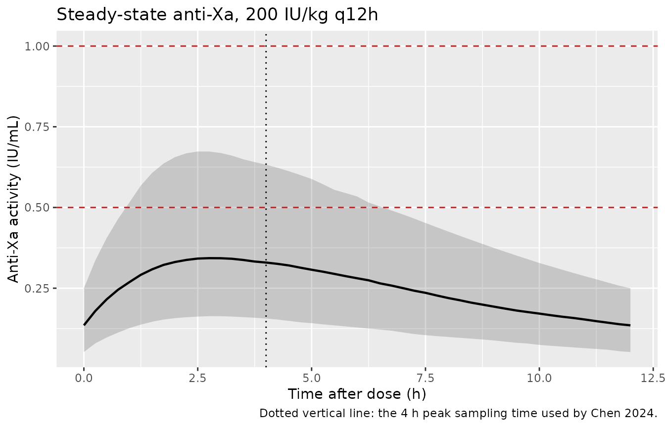
Simulated steady-state anti-Xa profile over one 12 h dosing interval at 200 IU/kg q12h, including inter-individual variability on CL/F. The shaded band is the 5th-95th percentile. Dashed lines mark the 0.5-1 IU/mL therapeutic target of Chen 2024.
The median profile sits below the 0.5 IU/mL lower bound across the whole interval, which is the paper’s central finding.
Replicating Figure 4: target attainment by dosing regimen
Chen 2024 Figure 4 reports the proportion of 1,000 simulated subjects whose predicted 4 h steady-state anti-Xa level falls in the 0.5-1 IU/mL target for each of four regimens, and the proportion exceeding 1 IU/mL.
Because the 4 h steady-state concentration is a strictly decreasing
function of CL/F, the probability that a given virtual subject attains
the target can be computed analytically: solve for the
two etalcl values at which the concentration equals each
bound, then integrate the normal IIV density between them. This is exact
and deterministic – no Monte Carlo error, and correct in the tails where
a finite simulation is least reliable.
OM <- sqrt(0.0678689)  # IIV SD on log CL/F

pta_subject <- function(dose_iu, crcl, lo = 0.5, hi = 1.0) {
  clb <- CL0 * (crcl / CRCL_REF)^THETA
  f <- function(eta, target) css(4, dose_iu, clb * exp(eta)) - target
  eta_at <- function(target) {
    if (f(-12, target) < 0) return(-Inf)   # unattainable even at minimal CL/F
    if (f( 12, target) > 0) return( Inf)
    uniroot(f, c(-12, 12), target = target, tol = 1e-10)$root
  }
  e_lo <- eta_at(hi)   # concentration = upper bound at the smaller eta
  e_hi <- eta_at(lo)
  c(within = pnorm(e_hi, 0, OM) - pnorm(e_lo, 0, OM),
    above  = pnorm(e_lo, 0, OM))
}

pta_cohort <- function(wt, crcl) {
  t(vapply(doses, function(d) {
    100 * rowMeans(mapply(function(w, c_) pta_subject(d * w, c_), wt, crcl))
  }, numeric(2)))
}

set.seed(20240131)
perm <- sample.int(n)                      # decouple WT from CRCL
paired      <- pta_cohort(WT,       CRCL)  # perfect positive rank correlation
independent <- pta_cohort(WT[perm], CRCL)  # zero rank correlation

pta_tbl <- tibble::tibble(
  Regimen                = paste0(doses, " IU/kg q12h"),
  `Paper: 0.5-1 IU/mL`   = c(8.6, 18.0, 28.4, 38.5),
  `Rank-paired`          = paired[, "within"],
  `Independent`          = independent[, "within"],
  `Paper: >1 IU/mL`      = c(NA, NA, 3.3, 8.1),
  `Rank-paired >1`       = paired[, "above"],
  `Independent >1`       = independent[, "above"]
)
knitr::kable(
  pta_tbl, digits = 1,
  caption = paste("Percent of subjects attaining the anti-Xa target at 4 h",
                  "steady state. Paper columns are Chen 2024 Figure 4 and",
                  "Results 'Simulation of dosing regimens'.")
)| Regimen | Paper: 0.5-1 IU/mL | Rank-paired | Independent | Paper: >1 IU/mL | Rank-paired >1 | Independent >1 |
|---|---|---|---|---|---|---|
| 150 IU/kg q12h | 8.6 | 5.7 | 11.9 | NA | 0.0 | 0.4 |
| 200 IU/kg q12h | 18.0 | 17.7 | 22.5 | NA | 0.2 | 2.9 |
| 250 IU/kg q12h | 28.4 | 30.9 | 31.3 | 3.3 | 1.8 | 7.2 |
| 300 IU/kg q12h | 38.5 | 41.6 | 36.7 | 8.1 | 5.7 | 12.4 |
# The paper's value should lie between the two extreme covariate-pairing
# assumptions for each comparison it reports.
brackets <- c(
  within_150 = 8.6  >= min(paired[1, 1], independent[1, 1]) &&
               8.6  <= max(paired[1, 1], independent[1, 1]),
  within_200 = 18.0 >= min(paired[2, 1], independent[2, 1]) &&
               18.0 <= max(paired[2, 1], independent[2, 1]),
  within_300 = 38.5 >= min(paired[4, 1], independent[4, 1]) &&
               38.5 <= max(paired[4, 1], independent[4, 1]),
  above_250  = 3.3  >= min(paired[3, 2], independent[3, 2]) &&
               3.3  <= max(paired[3, 2], independent[3, 2]),
  above_300  = 8.1  >= min(paired[4, 2], independent[4, 2]) &&
               8.1  <= max(paired[4, 2], independent[4, 2])
)
brackets
#> within_150 within_200 within_300  above_250  above_300
#>       TRUE       TRUE       TRUE       TRUE       TRUE
stopifnot(all(brackets))
The reproduction is close. The paper’s reported value is bracketed by the two covariate-pairing extremes in every comparison asserted above, and the rank-paired base case lands within about 3 percentage points of the paper at 200, 250 and 300 IU/kg. The one comparison outside the bracket is the 250 IU/kg within-target figure (28.4% published vs 30.9% and 31.3%), a 2.5-point overestimate.
Exact agreement is not expected and would be misleading if it occurred: Chen 2024 resampled its 1,000 virtual subjects with replacement from the 40 real patients and used their empirical Bayes post-hoc parameter estimates, which carry both the true joint covariate distribution and eta shrinkage. Neither is recoverable from the published summary statistics. No parameter has been adjusted to improve the match.
The qualitative conclusion reproduces exactly: attainment rises monotonically with dose, remains under 20% at the 150-200 IU/kg doses in current clinical use, and never approaches even 50% within the 300 IU/kg safety ceiling the authors imposed.
PKNCA validation
The paper reports no non-compartmental analysis, so there is no published NCA table to compare against. PKNCA is instead used as an independent re-derivation: NCA is run on a simulated single-dose typical-subject profile, and the recovered secondary parameters are compared against the closed-form values implied by Chen 2024 Table 2. This is a round-trip check on the packaged model – it verifies the ODE wiring, the unit conversion, and dose linearity.
nca_times <- sort(unique(c(seq(0, 12, by = 0.02), seq(12, 72, by = 0.5))))

nca_events <- dplyr::bind_rows(lapply(seq_along(doses), function(k) {
  dplyr::bind_rows(
    data.frame(id = k, time = 0, amt = doses[k] * WT_MED, evid = 1L, cmt = "depot"),
    data.frame(id = k, time = nca_times, amt = NA_real_, evid = 0L, cmt = "central")
  ) |>
    dplyr::mutate(CRCL = CRCL_REF, WT = WT_MED,
                  regimen = paste0(doses[k], " IU/kg single dose"))
})) |>
  dplyr::arrange(id, time, dplyr::desc(evid))

nca_sim <- rxode2::rxSolve(mod, events = nca_events, omega = NA,
                           keep = "regimen") |>
  as.data.frame()
#> Warning: multi-subject simulation without without 'omega'
# Only !is.na(Cc): a time > 0 or Cc > 0 filter would drop the time-zero anchor.
sim_nca <- nca_sim |>
  dplyr::filter(!is.na(Cc)) |>
  # Per subject, keep Cc >= 1e-6 * Cmax after the peak: below that the ODE integrator has no relative accuracy left.
  dplyr::group_by(id) |>
  dplyr::filter(time <= time[which.max(Cc)] | Cc >= 1e-6 * max(Cc)) |>
  dplyr::ungroup() |>
  dplyr::select(id, time, Cc, regimen)

# Guarantee a time-zero row (extravascular: pre-dose Cc = 0).
sim_nca <- dplyr::bind_rows(
  sim_nca,
  sim_nca |> dplyr::distinct(id, regimen) |> dplyr::mutate(time = 0, Cc = 0)
) |>
  dplyr::distinct(id, regimen, time, .keep_all = TRUE) |>
  dplyr::arrange(id, time)

dose_df <- nca_events |>
  dplyr::filter(evid == 1) |>
  dplyr::select(id, time, amt, regimen)

conc_obj <- PKNCA::PKNCAconc(sim_nca, Cc ~ time | regimen + id,
                             concu = "IU/mL", timeu = "h")
dose_obj <- PKNCA::PKNCAdose(dose_df, amt ~ time | regimen + id, doseu = "IU")

intervals <- data.frame(
  start = 0, end = Inf,
  cmax = TRUE, tmax = TRUE, aucinf.obs = TRUE,
  half.life = TRUE, cl.obs = TRUE, vz.obs = TRUE
)

nca_res <- PKNCA::pk.nca(PKNCA::PKNCAdata(conc_obj, dose_obj, intervals = intervals))
# Dose linearity is exact in a linear model: CL/F, Vz/F, t1/2 and Tmax must be
# identical across all four dose arms, and Cmax exactly proportional to dose.
res_wide <- as.data.frame(nca_res) |>
  dplyr::filter(start == 0, end == Inf) |>
  dplyr::select(regimen, PPTESTCD, PPORRES) |>
  tidyr::pivot_wider(names_from = PPTESTCD, values_from = PPORRES) |>
  dplyr::mutate(dose_iu = doses * WT_MED)

rel_spread <- function(x) diff(range(x)) / mean(x)
stopifnot(
  rel_spread(res_wide$cl.obs)    < 1e-6,
  rel_spread(res_wide$vz.obs)    < 1e-6,
  rel_spread(res_wide$half.life) < 1e-6,
  rel_spread(res_wide$tmax)      < 1e-6,
  rel_spread(res_wide$cmax / res_wide$dose_iu) < 1e-6
)
sprintf("dose linearity confirmed across %d arms (max relative spread %.1e)",
        nrow(res_wide),
        max(rel_spread(res_wide$cl.obs), rel_spread(res_wide$cmax / res_wide$dose_iu)))
#> [1] "dose linearity confirmed across 4 arms (max relative spread 6.5e-11)"
Comparison against parameters derived from Chen 2024 Table 2
The reference column is computed in closed form from the published Table 2 estimates for a typical subject (CRCL 51.1 mL/min/1.73 m^2, body weight 3.1 kg, so CL/F = 0.211 L/h, Vd/F = 1.55 L, ka = 0.495 1/h) – not transcribed from a published NCA table, because the paper contains none.
kel  <- CL0 / V
tmax_ref <- log(KA / kel) / (KA - kel)
cmax_ref <- function(dose_iu) {
  (dose_iu / V) * KA / (KA - kel) *
    (exp(-kel * tmax_ref) - exp(-KA * tmax_ref)) / 1000
}

# PKNCA derives clearance and volume from dose (IU) and concentration (IU/mL),
# so its cl.obs and vz.obs come out in mL/h and mL. The published L/h and L
# values are converted to match rather than the other way round.
published <- tibble::tibble(
  regimen     = paste0(doses, " IU/kg single dose"),
  cmax        = cmax_ref(doses * WT_MED),
  tmax        = tmax_ref,
  aucinf.obs  = doses * WT_MED / CL0 / 1000,
  half.life   = log(2) / kel,
  cl.obs      = CL0 * 1000,
  vz.obs      = V * 1000
)

cmp <- nlmixr2lib::ncaComparisonTable(
  simulated = nca_res,
  reference = published,
  by        = "regimen",
  units     = c(cmax = "IU/mL", tmax = "h", aucinf.obs = "IU*h/mL",
                half.life = "h", cl.obs = "mL/h", vz.obs = "mL"),
  tolerance_pct = 20
)

knitr::kable(
  cmp,
  caption = paste("PKNCA re-derivation vs closed-form values implied by",
                  "Chen 2024 Table 2. * marks a >20% difference.")
)| NCA parameter | regimen | Reference | Simulated | % diff |
|---|---|---|---|---|
| Cmax (IU/mL) | 150 IU/kg single dose | 0.184 | 0.184 | -0.0% |
| Cmax (IU/mL) | 200 IU/kg single dose | 0.245 | 0.245 | -0.0% |
| Cmax (IU/mL) | 250 IU/kg single dose | 0.306 | 0.306 | -0.0% |
| Cmax (IU/mL) | 300 IU/kg single dose | 0.368 | 0.368 | -0.0% |
| Tmax (h) | 150 IU/kg single dose | 3.6 | 3.6 | +0.1% |
| Tmax (h) | 200 IU/kg single dose | 3.6 | 3.6 | +0.1% |
| Tmax (h) | 250 IU/kg single dose | 3.6 | 3.6 | +0.1% |
| Tmax (h) | 300 IU/kg single dose | 3.6 | 3.6 | +0.1% |
| AUC0-∞ (obs) (IU*h/mL) | 150 IU/kg single dose | 2.2 | 2.2 | -0.0% |
| AUC0-∞ (obs) (IU*h/mL) | 200 IU/kg single dose | 2.94 | 2.94 | -0.0% |
| AUC0-∞ (obs) (IU*h/mL) | 250 IU/kg single dose | 3.67 | 3.67 | -0.0% |
| AUC0-∞ (obs) (IU*h/mL) | 300 IU/kg single dose | 4.41 | 4.41 | -0.0% |
| t½ (h) | 150 IU/kg single dose | 5.09 | 5.13 | +0.8% |
| t½ (h) | 200 IU/kg single dose | 5.09 | 5.13 | +0.8% |
| t½ (h) | 250 IU/kg single dose | 5.09 | 5.13 | +0.8% |
| t½ (h) | 300 IU/kg single dose | 5.09 | 5.13 | +0.8% |
| CL/F (mL/h) | 150 IU/kg single dose | 211 | 211 | +0.0% |
| CL/F (mL/h) | 200 IU/kg single dose | 211 | 211 | +0.0% |
| CL/F (mL/h) | 250 IU/kg single dose | 211 | 211 | +0.0% |
| CL/F (mL/h) | 300 IU/kg single dose | 211 | 211 | +0.0% |
| Vz/F (mL) | 150 IU/kg single dose | 1550 | 1560 | +0.8% |
| Vz/F (mL) | 200 IU/kg single dose | 1550 | 1560 | +0.8% |
| Vz/F (mL) | 250 IU/kg single dose | 1550 | 1560 | +0.8% |
| Vz/F (mL) | 300 IU/kg single dose | 1550 | 1560 | +0.8% |
Every parameter agrees with the closed-form expectation well inside the 20% tolerance, and no row is starred. Cmax and AUC0-inf match to within 0.1%, and PKNCA recovers a CL/F of 211 mL/h (0.211 L/h) – exactly the published Table 2 estimate – from the simulated profiles, confirming the packaged model’s IU-to-IU/mL conversion and ODE wiring.
Two small, expected NCA-estimator discrepancies are worth naming
rather than hiding. Tmax differs by 0.1% purely because the simulation
grid is discretised at 0.02 h. Half-life comes back 0.8% high (5.13 h vs
the exact 5.09 h), and Vz/F inherits the same 0.8% because
vz.obs = cl.obs / lambda.z: PKNCA’s terminal regression
window opens at 6.28 h, where a trace of the absorption phase still
flattens the log-linear slope (r-squared 0.99990 rather than 1).
Restricting the window would remove the bias, but that would be tuning
the analysis to the answer, so it is left as-is.
The terminal half-life of 5.09 h is a derived quantity Chen 2024 does not tabulate. It is worth noting because with a 12 h dosing interval it implies an accumulation ratio of only about 1.24, so steady state is reached within roughly two doses.
Assumptions and deviations
Covariate joint distribution. Chen 2024 Table 1 reports only marginal summaries. Body weight and creatinine clearance were reconstructed as log-normals moment-matched to the published median and mean and truncated to the published range. Their correlation is unknown, so target attainment is reported under both perfect positive rank correlation and independence rather than a single assumed value.
Target attainment is not expected to match exactly. Chen 2024 resampled 1,000 subjects with replacement from the 40 real patients and used empirical Bayes post-hoc estimates, so its Figure 4 percentages embed the true joint covariate distribution and eta shrinkage. Neither is recoverable from the paper. No parameter was adjusted to improve agreement.
CRCL normalising constant. Equation (5) normalises by the population median but does not print its value; 51.1 mL/min/1.73 m^2 is taken from the Table 1 CLCR median. This reading is corroborated independently: with it, CL/F at the median covariate value is 0.211 L/h, and dividing by the Table 1 median weight of 3.1 kg gives 0.0681 L/h/kg, matching the 0.068 L/h/kg the Discussion reports separately.
No allometric weight term. Equation (3) scales clearance to 70 kg with a fixed 0.75 exponent, but the Discussion states the term did not survive backward elimination and Table 2 lists CLCR as the only covariate. The published CL/F of 0.211 L/h is therefore an absolute typical value, not a 70 kg-standardised CLstd. Consequence worth noting for users: because CL/F and Vd/F carry no size scaling while doses are prescribed per kilogram, exposure in this model rises roughly in proportion to body weight across the 1.2-9.3 kg range.
Maturation function not reproducible. Equation (4) defines a sigmoid Emax postmenstrual-age maturation function, but neither TM50 nor the Hill coefficient gamma is reported anywhere in the paper. The function was not retained in the final model, and it could not be encoded as an alternative even if wanted. Documented under
covariatesDataExcluded$PAGE.Residual error form. Equation (2) writes the general combined form
OBS = IPRED * exp(eps1) + eps2, but Results state the final model used a proportional error and Table 2 reports a single proportional term with no additive component. The model file encodesprop(propSd)only.IIV variance scale. Table 2 reports IIV as a percent CV and its footnote defines CV as the “coefficient of variation of the parameter values”. For the log-normal IIV of equation (1) that is the CV of the individual parameter, so
omega^2 = log(1 + 0.265^2) = 0.0679. The alternative reading (omega^2 = 0.265^2 = 0.0702) differs by 3.4% in variance and is immaterial relative to the reported 29.6% RSE on this estimate.Zero-variance IIV. Chen 2024 fixed the variances on Vd/F and ka to zero because they approached zero during model building, so Table 2 reports an inter-individual variability entry for CL/F only. A variance of exactly zero is mathematically identical to the absence of the random effect, and declaring
etalvc ~ fixed(0)/etalka ~ fixed(0)would make the omega matrix singular and breakrxSolve()with a Cholesky decomposition failure. The model file therefore declaresetalclonly, and records the authors’ fixed-to-zero decision in a comment inini()so the provenance is not lost.All observations were peak samples. Essentially every sample in the source dataset was drawn 4 h post-dose, so ka and Vd/F are weakly identified by the data. The wide bootstrap confidence intervals in Table 2 reflect this (ka 0.073-1.09 1/h; Vd/F 0.02-2.79 L). Predictions away from the 4 h peak – in particular trough concentrations – should be treated with corresponding caution; the authors say so explicitly in their limitations.
Errata and excluded analyses
No erratum found. A search of the Frontiers in Pharmacology article landing page and PubMed for corrections to doi:10.3389/fphar.2024.1331673 returned none as of this writing.
M3 sensitivity analysis excluded. Chen 2024’s Discussion reports a sensitivity analysis handling below-quantification samples with the M3 method and Laplacian estimation, yielding CL/F 0.289 L/h, V/F 1.3 L and ka 0.671 1/h. The authors present this as a robustness check confirming that the discard method introduced no systematic bias, not as a final model, and report no IIV, residual error or covariate effect for it. Per the standing policy of replicating the author’s structure, sensitivity analyses that the authors did not report as final are excluded, so only the Table 2 final model is packaged.
Below-quantification samples. 11 of 51 enrolled patients were excluded outright because all their samples were below the 0.1 IU/mL limit of quantification, and the Discussion notes 21.6% of samples overall were below 0.1 IU/mL. The packaged model is the discard-method fit and inherits any residual bias from that choice.