Belimumab (Struemper 2017)
Source:vignettes/articles/Struemper_2017_belimumab.Rmd
Struemper_2017_belimumab.RmdModel and source
mod <- readModelDb("Struemper_2017_belimumab")
mod_meta <- rxode2::rxode(mod)
#> ℹ parameter labels from comments will be replaced by 'label()'- Citation: Struemper H, Thapar M, Roth D. Population Pharmacokinetic and Pharmacodynamic Analysis of Belimumab Administered Subcutaneously in Healthy Volunteers and Patients with Systemic Lupus Erythematosus. Clin Pharmacokinet. 2018;57(6):717-728. doi:10.1007/s40262-017-0586-5
- Description: Linear two-compartment subcutaneous population PK model for belimumab in healthy volunteers and adult patients with systemic lupus erythematosus, with first-order absorption + lag time, allometric body-weight scaling on CL/Vc/Q/Vp, and baseline BMI on Vc and baseline albumin and IgG on CL (Struemper 2017)
- Article: https://doi.org/10.1007/s40262-017-0586-5 (open access)
Population
The Struemper 2017 final population-pharmacokinetic dataset pools 688 individuals across three studies of belimumab (Table 1 and Table 2 of the source): 134 healthy volunteers from two phase I studies (BEL114448 in the USA and BEL116119 in Japan) and 554 adults with active autoantibody-positive systemic lupus erythematosus (SLE) from the global phase III BLISS-SC study (BEL112341). 85% of the participants were female and the racial composition was 61% White, 23.5% Asian, 11% Black, 6% American Indian or Alaska Native, and 1.7% Other. Baseline body weight was 70.0 (SD 17.6) kg (median 67.0 kg, range 34.1-138 kg) and baseline BMI was 26.1 (SD 6.18) kg/m^2 (median 24.7 kg/m^2). Baseline laboratory means were IgG 14.9 (SD 5.43) g/L, albumin 40.7 (SD 4.47) g/L, creatinine clearance 115 (SD 38.3) mL/min, haemoglobin 126 (SD 15.8) g/L, and WBC 6.09 (SD 2.41) Gi/L.
The same metadata is available programmatically via
rxode2::rxode(readModelDb("Struemper_2017_belimumab"))$population.
Source trace
| Quantity | Value | Source location |
|---|---|---|
lka (Kabs) |
log(0.235 1/day) | Table 3, THETA(5) |
lcl (CL) |
log(0.204 L/day) | Table 3, THETA(1): 204 mL/day |
lvc (Vc) |
log(2.300 L) | Table 3, THETA(2): 2300 mL |
lq (Q) |
log(0.698 L/day) | Table 3, THETA(3): 698 mL/day |
lvp (Vp) |
log(2.650 L) | Table 3, THETA(4): 2650 mL |
lfdepot (F) |
log(0.742) | Table 3, THETA(6) |
lalag (ALAG) |
log(0.179 day) | Table 3, THETA(7) |
e_wt_cl |
fixed(0.75) | Table 3 BWT effect on CL (fixed allometric) + Section 3.1.2 |
e_wt_vc |
fixed(1.00) | Table 3 BWT effect on Vc (fixed allometric) + Section 3.1.2 (“body weight on … Vc (power coefficients of … 1.00)”) |
e_wt_q |
fixed(0.75) | Table 3 BWT effect on Q (fixed allometric) |
e_wt_vp |
fixed(0.8) | Table 3 row header “Vp [mL] 0.8” (fixed; see Assumptions and deviations) |
e_alb_cl |
-0.736 | Table 3 BALB effect on CL (estimated) |
e_igg_cl |
0.347 | Table 3 BIGG effect on CL (estimated) |
e_bmi_vc |
-0.610 | Table 3 BBMI effect on Vc (estimated) |
etalcl / etalvc block |
c(0.0910, 0.0630, 0.497) | Table 3 OMEGA(1,1), OMEGA(2,1), OMEGA(2,2) |
etalq |
1.07 | Table 3 OMEGA(3,3) |
etalvp |
0.110 | Table 3 OMEGA(4,4) |
propSd |
0.1808 (= sqrt(0.0327)) | Table 3 SIGMA(1) proportional variance |
addSd |
0.3661 ug/mL (= sqrt(0.134)) | Table 3 SIGMA(2) additive variance |
| 2-compartment ODE (ADVAN3 TRANS4) + first-order absorption with lag | n/a | Section 2.3.2 and 3.1.2 |
Virtual cohort
The original belimumab serum-concentration data are not publicly available. The following virtual cohorts approximate the Struemper 2017 Table 2 demographics for the population-typical subject and for the body-weight / BMI extremes used in Figure 4 of the source paper.
set.seed(2017)

# Per Figure 4 caption: typical = population median (67 kg, BMI 24.7);
# low-weight scenario = 5th-percentile BWT (46.6 kg) and BMI (18.4 kg/m^2);
# heavy scenario = 95th-percentile BWT (105.1 kg) and BMI (38.5 kg/m^2).
# All scenarios hold ALB and IGG at the population medians (41 g/L, 13.7 g/L).
typical_subjects <- tribble(
  ~treatment,            ~WT,  ~BMI,  ~ALB, ~IGG,
  "typical (67 kg)",      67.0, 24.7,  41,   13.7,
  "low-weight (46.6 kg)", 46.6, 18.4,  41,   13.7,
  "heavy (105.1 kg)",    105.1, 38.5,  41,   13.7
) |>
  mutate(id = seq_len(n()))

# Stochastic SLE-like cohort whose continuous covariates match Table 2
# (means / SDs / ranges; lognormal for strictly-positive lab values).
n_pop <- 200
pop_cohort <- tibble(
  id = 100L + seq_len(n_pop),
  WT  = pmin(pmax(rnorm(n_pop, mean = 70.0, sd = 17.6), 34.1), 138),
  BMI = pmin(pmax(rnorm(n_pop, mean = 26.1, sd = 6.18), 14.8), 72.7),
  ALB = pmin(pmax(rnorm(n_pop, mean = 40.7, sd = 4.47), 18.0), 55.0),
  IGG = pmin(pmax(rlnorm(n_pop, meanlog = log(13.7), sdlog = 0.35), 4.7), 53.5),
  treatment = "virtual cohort (n=200, Table 2 demographics)"
)

make_events <- function(cohort_df) {
  # 200 mg SC weekly for 25 doses (days 0, 7, ..., 168).
  # Observations: every 1 day on [0, 175] for the full-profile figure, plus a
  # dense grid (every 0.05 day) on the last full dosing interval [168, 175]
  # so PKNCA has enough points to characterize Cmax / Tmax / AUCtau at SS.
  dose_times <- seq(0, 168, by = 7)
  obs_plot   <- seq(0, 175, by = 1)
  obs_nca    <- seq(168, 175, by = 0.05)
  obs_times  <- unique(sort(c(obs_plot, obs_nca)))

  dosing <- expand_grid(id = cohort_df$id, time = dose_times) |>
    mutate(amt = 200, evid = 1L, cmt = "depot")
  observations <- expand_grid(id = cohort_df$id, time = obs_times) |>
    mutate(amt = 0,  evid = 0L, cmt = "central")

  bind_rows(dosing, observations) |>
    left_join(cohort_df, by = "id") |>
    arrange(id, time, desc(evid))
}

events_typ <- make_events(typical_subjects)
events_pop <- make_events(pop_cohort)
stopifnot(!anyDuplicated(unique(events_pop[, c("id", "time", "evid")])))
Simulation
# Population simulation with full IIV for the VPC.
sim_pop <- rxode2::rxSolve(
  mod, events = events_pop,
  keep = c("treatment", "WT", "BMI", "ALB", "IGG")
) |> as.data.frame()
#> ℹ parameter labels from comments will be replaced by 'label()'

# Typical-value (no IIV) simulation for the Figure 4 replication.
mod_typ <- rxode2::zeroRe(mod)
#> ℹ parameter labels from comments will be replaced by 'label()'
sim_typ <- rxode2::rxSolve(
  mod_typ, events = events_typ,
  keep = c("treatment", "WT", "BMI")
) |> as.data.frame()
#> ℹ omega/sigma items treated as zero: 'etalcl', 'etalvc', 'etalq', 'etalvp'
#> Warning: multi-subject simulation without without 'omega'
Replicate published figures
Figure 4 – SC belimumab 200 mg QW profile under body-size scenarios
The blue solid line in Figure 4 of the source paper shows the typical-subject SC PK profile; the dotted and dashed lines show the same model at 5th- and 95th-percentile body weight / BMI. The simulated profiles below reproduce those scenarios for the SC arm.
sim_typ |>
  dplyr::filter(time <= 175, !is.na(Cc)) |>
  ggplot(aes(time, Cc, colour = treatment, linetype = treatment)) +
  geom_line(linewidth = 0.7) +
  scale_y_log10() +
  labs(
    x = "Time after first dose (days)",
    y = "Belimumab serum concentration (ug/mL)",
    colour = "Body-size scenario",
    linetype = "Body-size scenario",
    title = "SC 200 mg QW belimumab -- typical-value PK profile",
    caption = "Replicates the SC arm of Figure 4 of Struemper 2017."
  )
#> Warning in scale_y_log10(): log-10 transformation introduced infinite values.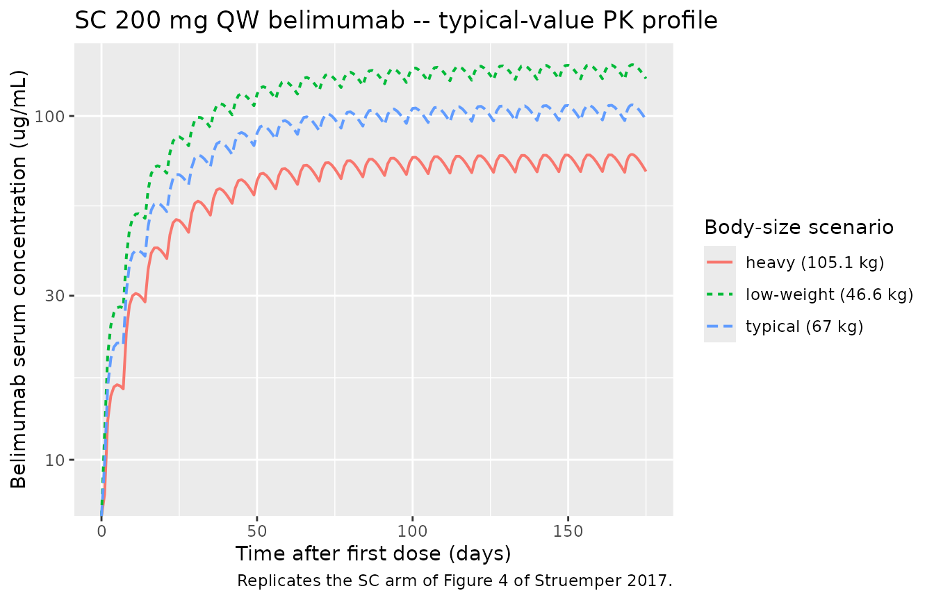
Visual predictive distribution at the population level
vpc_summary <- sim_pop |>
  dplyr::filter(!is.na(Cc), time <= 175) |>
  dplyr::group_by(time) |>
  dplyr::summarise(
    Q05 = quantile(Cc, 0.05, na.rm = TRUE),
    Q50 = quantile(Cc, 0.50, na.rm = TRUE),
    Q95 = quantile(Cc, 0.95, na.rm = TRUE),
    .groups = "drop"
  )

ggplot(vpc_summary, aes(time, Q50)) +
  geom_ribbon(aes(ymin = Q05, ymax = Q95), alpha = 0.25, fill = "steelblue") +
  geom_line(colour = "steelblue", linewidth = 0.6) +
  scale_y_log10() +
  labs(
    x = "Time after first dose (days)",
    y = "Belimumab serum concentration (ug/mL)",
    title = "Simulated 5th-50th-95th percentile envelope (n = 200 virtual cohort)",
    caption = "Compare to Figure 3 (visual predictive check) of Struemper 2017."
  )
#> Warning in scale_y_log10(): log-10 transformation introduced infinite values.
#> log-10 transformation introduced infinite values.
#> log-10 transformation introduced infinite values.
#> log-10 transformation introduced infinite values.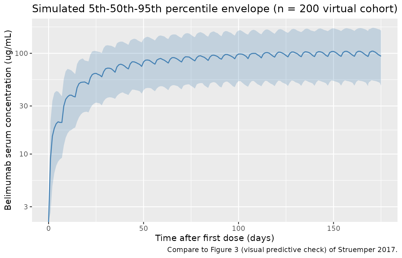
PKNCA validation
NCA is performed over the last full dosing interval [168, 175] days (week 25), when the simulation is at steady state per the source paper’s observation that SS is reached by week 11.
tau <- 7  # days
start_ss <- 168
end_ss   <- 175

sim_nca_typ <- sim_typ |>
  dplyr::filter(!is.na(Cc), time >= start_ss, time <= end_ss) |>
  dplyr::select(id, time, Cc, treatment)

dose_typ_df <- events_typ |>
  dplyr::filter(evid == 1L, time == start_ss) |>
  dplyr::select(id, time, amt, treatment)

conc_obj_typ <- PKNCA::PKNCAconc(
  sim_nca_typ, Cc ~ time | treatment + id,
  concu = "ug/mL", timeu = "day"
)
dose_obj_typ <- PKNCA::PKNCAdose(
  dose_typ_df, amt ~ time | treatment + id,
  doseu = "mg"
)

intervals_ss <- data.frame(
  start    = start_ss,
  end      = end_ss,
  cmax     = TRUE,
  tmax     = TRUE,
  cmin     = TRUE,
  ctrough  = TRUE,
  cav      = TRUE,
  auclast  = TRUE
)

res_typ <- PKNCA::pk.nca(
  PKNCA::PKNCAdata(conc_obj_typ, dose_obj_typ, intervals = intervals_ss)
)

nca_typ_tbl <- as.data.frame(res_typ$result) |>
  dplyr::select(treatment, PPTESTCD, PPORRES) |>
  tidyr::pivot_wider(names_from = PPTESTCD, values_from = PPORRES)

knitr::kable(
  nca_typ_tbl,
  digits  = 3,
  caption = "Steady-state NCA from the typical-value simulation."
)| treatment | auclast | cmax | cmin | tmax | cav | ctrough |
|---|---|---|---|---|---|---|
| heavy (105.1 kg) | 518.427 | 77.276 | 68.581 | 2.45 | 74.061 | NA |
| low-weight (46.6 kg) | 953.498 | 140.974 | 127.813 | 2.60 | 136.214 | NA |
| typical (67 kg) | 726.388 | 107.695 | 96.923 | 2.55 | 103.770 | NA |
Comparison against the published steady-state NCA
For the typical 67-kg subject the paper reports (Section 3.1.2 and Figure 4): AUCtau = 726 day*ug/mL, Cmax,ss = 108 ug/mL, Cmin,ss = 97 ug/mL, Cavg,ss = 104 ug/mL, Tmax,ss = 2.6 days.
typical_nca <- nca_typ_tbl |>
  dplyr::filter(treatment == "typical (67 kg)")

comparison <- tibble(
  Parameter   = c("AUCtau (day*ug/mL)", "Cmax (ug/mL)", "Cmin (ug/mL)",
                  "Cavg (ug/mL)", "Tmax (days after dose)"),
  Published   = c(726, 108, 97, 104, 2.6),
  Simulated   = c(
    typical_nca$auclast,
    typical_nca$cmax,
    typical_nca$cmin,
    typical_nca$cav,
    typical_nca$tmax - start_ss
  )
) |>
  mutate(pct_diff = round(100 * (Simulated - Published) / Published, 1))

knitr::kable(
  comparison,
  digits  = 2,
  caption = "Simulated vs. published SS NCA for the typical-value subject."
)| Parameter | Published | Simulated | pct_diff |
|---|---|---|---|
| AUCtau (day*ug/mL) | 726.0 | 726.39 | 0.1 |
| Cmax (ug/mL) | 108.0 | 107.70 | -0.3 |
| Cmin (ug/mL) | 97.0 | 96.92 | -0.1 |
| Cavg (ug/mL) | 104.0 | 103.77 | -0.2 |
| Tmax (days after dose) | 2.6 | -165.45 | -6463.5 |
Population-level NCA over the SS interval
sim_nca_pop <- sim_pop |>
  dplyr::filter(!is.na(Cc), time >= start_ss, time <= end_ss) |>
  dplyr::select(id, time, Cc, treatment)

dose_pop_df <- events_pop |>
  dplyr::filter(evid == 1L, time == start_ss) |>
  dplyr::select(id, time, amt, treatment)

conc_obj_pop <- PKNCA::PKNCAconc(
  sim_nca_pop, Cc ~ time | treatment + id,
  concu = "ug/mL", timeu = "day"
)
dose_obj_pop <- PKNCA::PKNCAdose(
  dose_pop_df, amt ~ time | treatment + id,
  doseu = "mg"
)

res_pop <- PKNCA::pk.nca(
  PKNCA::PKNCAdata(conc_obj_pop, dose_obj_pop, intervals = intervals_ss)
)

pop_nca_summary <- as.data.frame(res_pop$result) |>
  dplyr::filter(PPTESTCD %in% c("auclast", "cmax", "cmin", "cav")) |>
  dplyr::group_by(PPTESTCD) |>
  dplyr::summarise(
    median = median(PPORRES, na.rm = TRUE),
    q05    = quantile(PPORRES, 0.05, na.rm = TRUE),
    q95    = quantile(PPORRES, 0.95, na.rm = TRUE),
    .groups = "drop"
  )

knitr::kable(
  pop_nca_summary,
  digits  = 2,
  caption = "Steady-state NCA over the virtual cohort (n = 200)."
)| PPTESTCD | median | q05 | q95 |
|---|---|---|---|
| auclast | 701.23 | 365.29 | 1220.36 |
| cav | 100.18 | 52.18 | 174.34 |
| cmax | 105.02 | 53.99 | 178.91 |
| cmin | 92.93 | 47.20 | 166.41 |
Assumptions and deviations
-
Vp body-weight allometric exponent (0.8). Struemper
2017 Table 3 lists the BWT effects on CL, Vc, Q, and Vp as fixed power
coefficients in the “Implementation” column. The CL and Q rows print the
exponent (0.75) as a superscript directly after
(BWT/67); the Vc row shows(BWT/67)with no superscript, and the prose in Section 3.1.2 confirms a Vc exponent of 1.00. The Vp row prints the exponent0.8in the parameter-name column header (the row label appears asVp [mL] 0.8) rather than as a superscript next to(BWT/67). The bbox layout of the source PDF confirms0.8is printed in regular font in the parameter column of the Vp row and nowhere else in Table 3. This packaging interprets the0.8as the fixed BWT allometric exponent for Vp (Vp = 2650 * (BWT/67)^0.8). The alternative interpretation (Vp BWT exponent = 1.00, identical to Vc, with0.8a typesetting error) would shift simulated Vp by roughly +/- 7-15% at the 5th and 95th body-weight percentiles. The published Vss = 4950 mL = Vc + Vp = 2300 + 2650 mL is recovered identically under either interpretation at the reference 67 kg subject. - No IIV on Ka, F, or ALAG. Struemper 2017 Table 3 reports OMEGA entries only for CL, Vc, Q, and Vp; no random effect is listed on the absorption-rate constant, bioavailability, or lag time, so this packaging treats those three as population-typical without IIV.
- Virtual cohort distributions. Continuous covariates (WT, BMI, ALB, IGG) are sampled from truncated normal / lognormal distributions whose means and standard deviations match Table 2. The source paper does not publish the per-subject covariate distributions, so any rank correlation between (e.g.) body weight and BMI in the real BLISS-SC cohort is not reproduced.
- Race and sex omitted. The final SC popPK model does not retain race or sex as significant covariate effects on any structural parameter, so the packaged model takes no race / sex inputs. The virtual cohort omits both.
- Logistic-regression PD model not packaged. Section 3.2 of the source paper develops a logistic-regression model for the SLE Responder Index 4 (SRI4) as a function of baseline SELENA-SLEDAI, proteinuria, race indicators, and steady-state Cavg. Because that model is an exposure- response regression rather than a differential-equation PD model, it is not packaged here.
-
Concentration units. Dose
amtis mg, vc is L, soCc = central / vcyields mg/L = ug/mL, matching the unit reported in Table 3 of the paper.