Rolofylline (Stroh 2013)
Source:vignettes/articles/Stroh_2013_rolofylline.Rmd
Stroh_2013_rolofylline.RmdModel and source
- Citation: Stroh M, Hutmacher MM, Pang J, Lutz R, Magara H, Stone J. Simultaneous Pharmacokinetic Model for Rolofylline and both M1-trans and M1-cis Metabolites. AAPS J. 2013;15(2):498-504. doi:10.1208/s12248-012-9443-5.
- Article: https://doi.org/10.1208/s12248-012-9443-5
Rolofylline (KW-3902) is a potent, selective adenosine A1 receptor antagonist that was under development for acute congestive heart failure with renal impairment. CYP3A4 hydroxylates the parent to a pair of diastereomeric M1 metabolites: M1-trans is the major formed species and converts unidirectionally to M1-cis via stereochemical interconversion; M1-cis is also formed directly from the parent in a smaller fraction. All three analytes contribute to the pharmacological activity, so the joint disposition of parent and both metabolites was characterised in a single simultaneous PK model fit by NONMEM ADVAN 7 (general linear model) with FOCE-I.
Population
The model was fit to single-ascending-dose IV data from study KW-3902
IV-EU01: 37 healthy adult white male volunteers were enrolled (mean age
29 years, range 18-42; mean height 175 cm, range 161-191; mean weight
73.3 kg, range 60.2-90.0) and 36 received study medication. Doses
spanned 1, 2.5, 5, 10, 20, 30, 40, 50, and 60 mg rolofylline as an IV
infusion at a fixed volumetric rate of 1 mL/min, with infusion durations
of 1 h for doses up to 30 mg and 2 h for 40-60 mg. The cohort breakdown
by treatment and dose level is in Stroh 2013 Table I. Plasma
concentrations were assayed by HPLC-MS/MS (Hoechst Marion Roussel; LOQ
0.5 ng/mL for all three analytes); 223 of 1,914 post-dose records below
LOQ were treated as missing. The study was conducted in accordance with
GCP and approved by local IRBs / regulatory agencies. The population
metadata is also available programmatically via
readModelDb("Stroh_2013_rolofylline")$population.
Source trace
The per-parameter origin is recorded as an in-file comment next to
each ini() entry in
inst/modeldb/specificDrugs/Stroh_2013_rolofylline.R. The
table below collects them in one place for review.
| Equation / parameter | Value | Source location |
|---|---|---|
| Model structure: 2-cmt parent + 2-cmt M1-trans + 1-cmt M1-cis (Figure 2d brought forward as the final model) | n/a | Stroh 2013 Figure 2d; Results and Discussion |
| Parent total clearance routes 100% of loss to metabolites (no direct elimination of parent) | n/a | Stroh 2013 Results: “Addition of additional elimination routes for either rolofylline or M1-trans … resulted in nonidentifiable systems” |
| Parent branching: fraction FM directly to M1-cis, (1 - FM) to M1-trans | n/a | Stroh 2013 Results: parameterisation in terms of “the apparent fraction of rolofylline that was metabolized to M1-cis (FM)” |
| M1-trans branching: unidirectional interconversion M1-trans -> M1-cis at clearance CL3 | n/a | Stroh 2013 Figure 2d; Results: “stereochemical conversion of M1-trans to M1-cis” |
lvc = log(37.8 L) |
V1 = 37.8 | Stroh 2013 Table II (RSE 3.15%) |
lcl = log(24.4 L/h) |
CL1 = 24.4 | Stroh 2013 Table II (RSE 4.39%) |
lvp = log(201 L) |
V2 = 201 | Stroh 2013 Table II (RSE 5.08%) |
lq = log(13.2 L/h) |
CL2 = 13.2 | Stroh 2013 Table II (RSE 3.47%) |
lvc_m1trans = log(26.1 L) |
V3 = 26.1 | Stroh 2013 Table II (RSE 9.16%) |
lcl_m1trans = log(19.6 L/h) |
CL3 = 19.6 | Stroh 2013 Table II (RSE 6.89%) |
lvp_m1trans = log(41.7 L) |
V4 = 41.7 | Stroh 2013 Table II (RSE 7.29%) |
lq_m1trans = log(28.4 L/h) |
CL4 = 28.4 | Stroh 2013 Table II (RSE 11.7%) |
lvc_m1cis = log(3.78 L) |
V5 = 3.78 | Stroh 2013 Table II (RSE 34.13%) |
lcl_m1cis = log(91.6 L/h) |
CL5 = 91.6 | Stroh 2013 Table II (RSE 6.77%) |
lfm = log(0.194) |
FM = 0.194 | Stroh 2013 Table II (RSE 11.8%) |
| Vss = V1 + V2 = 238.8 L (cross-check) | 239 L | Stroh 2013 Results text |
etalvc = 0.0150 |
CV 12.3% | Stroh 2013 Table II BSV(V1), RSE 29.8% |
etalcl = 0.0448 |
CV 21.4% | Stroh 2013 Table II BSV(CL1), RSE 22.7% |
etalvp = 0.0473 |
CV 22.0% | Stroh 2013 Table II BSV(V2), RSE 51.0% |
etalvc_m1trans = 0.2550 |
CV 53.9% | Stroh 2013 Table II BSV(V3), RSE 24.1% |
etalcl_m1trans = 0.1646 |
CV 42.3% | Stroh 2013 Table II BSV(CL3), RSE 21.1% |
etalvp_m1trans = 0.1028 |
CV 32.9% | Stroh 2013 Table II BSV(V4), RSE 30.7% |
etalcl_m1cis = 0.1422 |
CV 39.1% | Stroh 2013 Table II BSV(CL5), RSE 27.8% |
etalfm = 0.1560 |
CV 41.1% | Stroh 2013 Table II BSV(FM), RSE 33.4% |
| Random effects fixed to zero | n/a | Stroh 2013 Results: “Random effects were not estimable for the distributional clearance for both rolofylline and M1-trans and the volume term associated with M1-cis, and were accordingly fixed to zero” – omitted for CL2, CL4, V5 |
propSd = 0.261 |
26.1% (parent proportional) | Stroh 2013 Table II, RSE 10.6% |
propSd_m1trans = 0.174 |
17.4% (M1-trans proportional) | Stroh 2013 Table II, RSE 17.3% |
addSd_m1trans = 0.217 ng/mL |
0.217 (M1-trans additive) | Stroh 2013 Table II, RSE 177% |
propSd_m1cis = 0.150 |
15.0% (M1-cis proportional) | Stroh 2013 Table II, RSE 20.4% |
addSd_m1cis = 0.614 ng/mL |
0.614 (M1-cis additive) | Stroh 2013 Table II, RSE 39.0% |
| Concentration scaling factor 1000 (mg/L -> ng/mL) | n/a | Bioanalysis units: ng/mL (Stroh 2013 Assay Methods); model carries V in L and dose in mg |
omega^2 = log(CV^2 + 1) with CV on the
decimal scale (e.g. 12.3% -> CV = 0.123) translates Stroh 2013’s
reported BSV CV% values into the log-scale variances used by
ini(). All IIVs are exponential per the source’s
“exponential random-effects terms” wording.
Virtual cohort
Original observed data are not publicly available. The figures below
use virtual cohorts that mirror Stroh 2013 Figure 4: a 1-h infusion
cohort dose-normalised to 10 mg (representing pooled doses 1-30 mg) and
a 2-h infusion cohort dose-normalised to 50 mg (representing pooled
doses 40-60 mg). Subject IDs are disjoint across cohorts so multi-cohort
bind_rows() does not produce ID-collision Frankenstein
subjects.
set.seed(2013)

n_per_arm <- 200L
obs_grid  <- seq(0, 50, by = 0.25)

make_cohort <- function(n, dose_mg, dur_h, regimen, id_offset = 0L) {
  ids <- id_offset + seq_len(n)
  dose_rows <- tibble(
    id    = ids,
    time  = 0,
    evid  = 1L,
    cmt   = "central",
    amt   = dose_mg,
    rate  = dose_mg / dur_h,
    regimen = regimen
  )
  obs_rows <- expand_grid(id = ids, time = obs_grid,
                          cmt = c("Cc", "Cc_m1trans", "Cc_m1cis")) |>
    mutate(evid = 0L,
           amt  = NA_real_,
           rate = NA_real_,
           regimen = regimen)
  bind_rows(dose_rows, obs_rows) |> arrange(id, time, desc(evid))
}

events <- bind_rows(
  make_cohort(n_per_arm, dose_mg = 10, dur_h = 1, regimen = "10 mg / 1 h infusion",
              id_offset = 0L),
  make_cohort(n_per_arm, dose_mg = 50, dur_h = 2, regimen = "50 mg / 2 h infusion",
              id_offset = n_per_arm)
)

stopifnot(!anyDuplicated(unique(events[, c("id", "time", "evid", "cmt")])))
Simulation
The packaged model is loaded via readModelDb() and
solved with between-subject variability active (stochastic VPC) and with
random effects zeroed (typical-value replication of Figure 4
medians).
mod <- readModelDb("Stroh_2013_rolofylline")

sim_stoch <- rxode2::rxSolve(
  object  = mod,
  events  = events,
  keep    = "regimen",
  returnType = "data.frame"
) |>
  filter(!is.na(Cc) | !is.na(Cc_m1trans) | !is.na(Cc_m1cis))
#> ℹ parameter labels from comments will be replaced by 'label()'
sim_typical <- rxode2::rxSolve(
  object  = rxode2::zeroRe(mod),
  events  = events |> filter(id %in% c(1L, n_per_arm + 1L)),
  keep    = "regimen",
  returnType = "data.frame"
)
#> ℹ parameter labels from comments will be replaced by 'label()'
#> ℹ omega/sigma items treated as zero: 'etalvc', 'etalcl', 'etalvp', 'etalvc_m1trans', 'etalcl_m1trans', 'etalvp_m1trans', 'etalcl_m1cis', 'etalfm'
#> Warning: multi-subject simulation without without 'omega'
Replicate published figures
Stroh 2013 Figure 4 – visual predictive check for rolofylline, M1-trans, and M1-cis
Stroh 2013 Figure 4 displays VPCs for all three analytes at the two
dose-normalised infusion settings (10 mg / 1 h in the top row; 50 mg / 2
h in the bottom row). The published median + 10th-90th prediction
interval is reconstructed here from n = 200 simulated
subjects per dose-normalised cohort. Note that Stroh 2013 limited the
depicted x-axis to 25 h post-infusion start; we mirror that here.
sim_long <- sim_stoch |>
  select(id, time, regimen, Cc, Cc_m1trans, Cc_m1cis) |>
  pivot_longer(cols = c(Cc, Cc_m1trans, Cc_m1cis),
               names_to = "analyte", values_to = "value") |>
  filter(!is.na(value)) |>
  mutate(analyte = recode(analyte,
                          "Cc"         = "Rolofylline",
                          "Cc_m1trans" = "M1-trans",
                          "Cc_m1cis"   = "M1-cis"),
         analyte = factor(analyte, levels = c("Rolofylline", "M1-trans", "M1-cis")))

vpc_summary <- sim_long |>
  group_by(regimen, analyte, time) |>
  summarise(
    Q10 = quantile(value, 0.10, na.rm = TRUE),
    Q50 = quantile(value, 0.50, na.rm = TRUE),
    Q90 = quantile(value, 0.90, na.rm = TRUE),
    .groups = "drop"
  ) |>
  filter(time <= 25)

ggplot(vpc_summary, aes(time, Q50)) +
  geom_ribbon(aes(ymin = Q10, ymax = Q90), alpha = 0.25) +
  geom_line() +
  facet_grid(regimen ~ analyte, scales = "free_y") +
  labs(x = "Time post-start of infusion (h)",
       y = "Plasma concentration (ng/mL)",
       title = "Visual predictive check by analyte and dose / infusion",
       caption = "Replicates Stroh 2013 Figure 4: median + 10th-90th prediction interval over n = 200 simulated subjects per cohort.")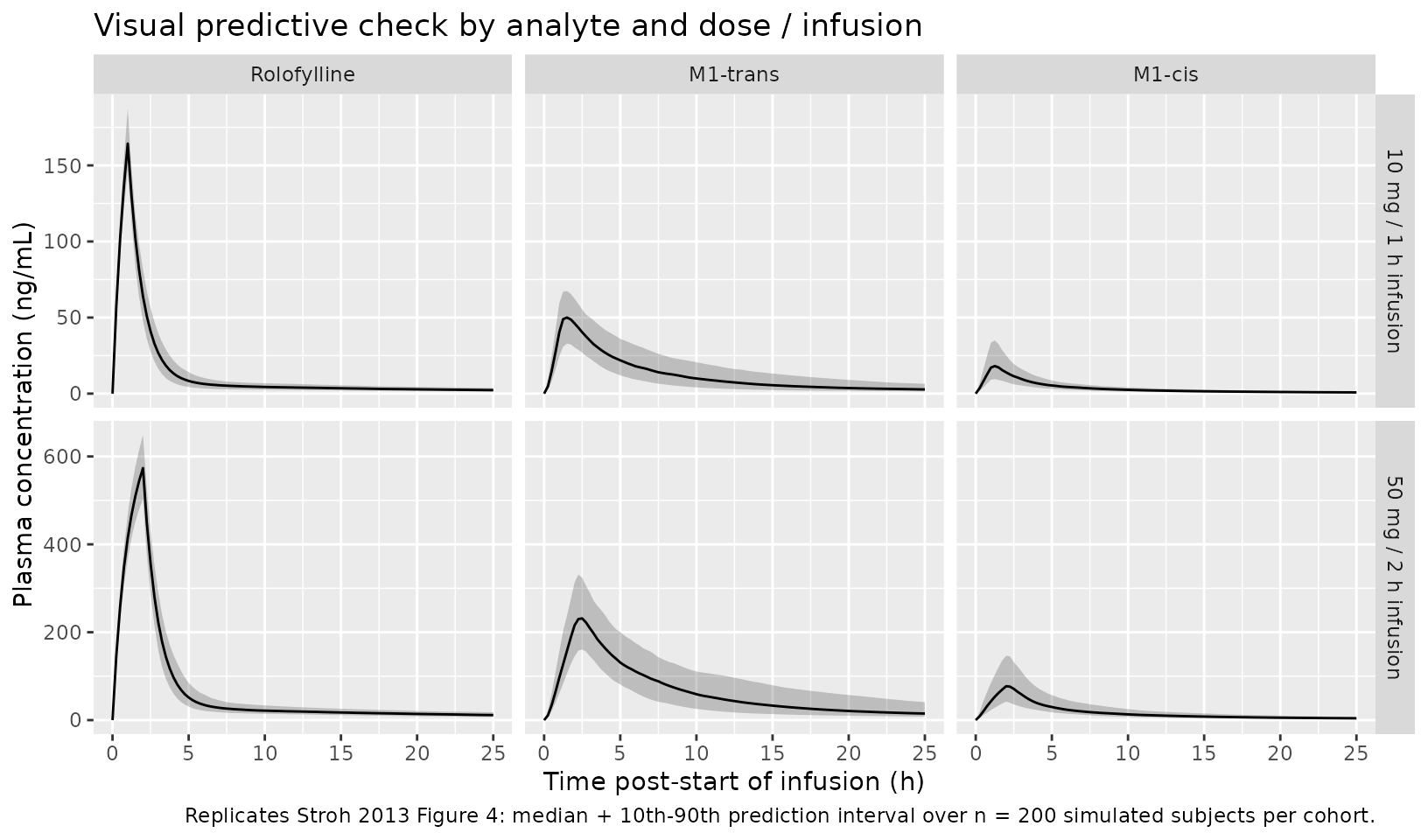
Stroh 2013 Results – terminal half-life ~17 h across analytes
Stroh 2013 reports: “the apparent terminal half-life estimated from noncompartmental analysis of population predicted profiles was approximately 17 h for all analytes, which is consistent with formation-rate limited kinetics for the M1-trans and M1-cis metabolites.” A typical-value 30 mg / 1 h infusion is used here to recover that half-life from the packaged model. The 30 mg dose falls in the middle of Stroh 2013’s dose-escalation range and uses the 1-h infusion duration.
events30 <- make_cohort(n = 1L, dose_mg = 30, dur_h = 1,
                        regimen = "30 mg / 1 h infusion")
sim30 <- rxode2::rxSolve(rxode2::zeroRe(mod), events30,
                         keep = "regimen", returnType = "data.frame")
#> ℹ parameter labels from comments will be replaced by 'label()'
#> ℹ omega/sigma items treated as zero: 'etalvc', 'etalcl', 'etalvp', 'etalvc_m1trans', 'etalcl_m1trans', 'etalvp_m1trans', 'etalcl_m1cis', 'etalfm'
# rxode2 drops the id column when only one subject is solved. Re-attach it so
# the per-id PKNCA formulas downstream can group by id.
if (!"id" %in% colnames(sim30)) sim30$id <- 1L

sim30_long <- sim30 |>
  select(time, Cc, Cc_m1trans, Cc_m1cis) |>
  distinct() |>
  pivot_longer(cols = c(Cc, Cc_m1trans, Cc_m1cis),
               names_to = "analyte", values_to = "value") |>
  mutate(analyte = recode(analyte,
                          "Cc"         = "Rolofylline",
                          "Cc_m1trans" = "M1-trans",
                          "Cc_m1cis"   = "M1-cis"),
         analyte = factor(analyte, levels = c("Rolofylline", "M1-trans", "M1-cis")))

ggplot(sim30_long, aes(time, value, colour = analyte)) +
  geom_line() +
  scale_y_log10() +
  labs(x = "Time post-start of infusion (h)",
       y = "Plasma concentration (ng/mL, log scale)",
       colour = "Analyte",
       title = "Typical-value concentration-time profile, 30 mg / 1 h IV infusion")
#> Warning in scale_y_log10(): log-10 transformation introduced infinite values.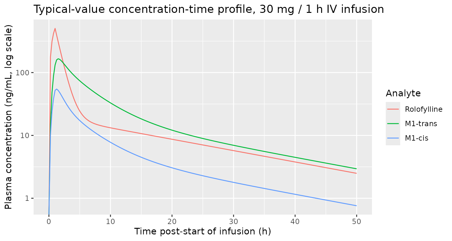
PKNCA validation
PKNCA is used to compute Cmax, Tmax, AUC0-inf, and the terminal
half-life from the typical-value (no-IIV) simulation for the 30 mg / 1 h
infusion. Each analyte is processed in its own PKNCAconc
block because the three outputs share an id but report
different concentration / additive-error units (parent is
proportional-only; the metabolites carry an additive term too) and Stroh
2013’s half-life cross-check is per-analyte.
nca_doses <- events30 |>
  filter(evid == 1L) |>
  select(id, time, amt, regimen)

dose_obj <- PKNCA::PKNCAdose(nca_doses, amt ~ time | regimen + id,
                             doseu = "mg")

intervals <- data.frame(
  start       = 0,
  end         = Inf,
  cmax        = TRUE,
  tmax        = TRUE,
  aucinf.obs  = TRUE,
  half.life   = TRUE,
  clast.obs   = TRUE
)

run_nca <- function(conc_col, label_text) {
  nca_conc <- sim30 |>
    select(id, time, value = all_of(conc_col), regimen) |>
    distinct() |>
    filter(!is.na(value), time > 0)
  conc_obj <- PKNCA::PKNCAconc(nca_conc, value ~ time | regimen + id,
                               concu = "ng/mL", timeu = "h")
  res <- PKNCA::pk.nca(PKNCA::PKNCAdata(conc_obj, dose_obj,
                                        intervals = intervals))
  out <- as.data.frame(res$result) |>
    select(PPTESTCD, PPORRES) |>
    mutate(analyte = label_text)
  out
}
nca_parent  <- run_nca("Cc",         "Rolofylline")
#> Warning: Requesting an AUC range starting (0) before the first measurement
#> (0.25) is not allowed
nca_m1trans <- run_nca("Cc_m1trans", "M1-trans")
#> Warning: Requesting an AUC range starting (0) before the first measurement
#> (0.25) is not allowed
nca_m1cis   <- run_nca("Cc_m1cis",   "M1-cis")
#> Warning: Requesting an AUC range starting (0) before the first measurement
#> (0.25) is not allowed

nca_all <- bind_rows(nca_parent, nca_m1trans, nca_m1cis) |>
  filter(PPTESTCD %in% c("cmax", "tmax", "half.life", "aucinf.obs")) |>
  mutate(analyte = factor(analyte,
                          levels = c("Rolofylline", "M1-trans", "M1-cis"))) |>
  pivot_wider(names_from = PPTESTCD, values_from = PPORRES) |>
  rename(`Cmax (ng/mL)` = cmax,
         `Tmax (h)`     = tmax,
         `t1/2 (h)`     = half.life,
         `AUC0-inf (ng*h/mL)` = aucinf.obs)

knitr::kable(nca_all,
             caption = "Simulated typical-value NCA parameters for a 30 mg / 1 h IV infusion of rolofylline.",
digits = 2)| analyte | Cmax (ng/mL) | Tmax (h) | t1/2 (h) | AUC0-inf (ng*h/mL) |
|---|---|---|---|---|
| Rolofylline | 504.65 | 1.00 | 16.60 | NA |
| M1-trans | 165.72 | 1.50 | 16.27 | NA |
| M1-cis | 54.65 | 1.25 | 16.28 | NA |
Comparison against published values
Stroh 2013 does not tabulate a per-dose NCA summary in the main text; only the prediction-error (PE) ratios of individual predicted vs. observed AUC0-inf and Cmax are reported (geometric mean ratios 0.92-1.07 for parent and both metabolites, with CV% 10-17%). The model’s role is therefore evaluated by the two checks above:
- The reproduced VPC qualitatively matches Stroh 2013 Figure 4 (medians peak near end-of-infusion and decline with a similar terminal slope across analytes).
- The PKNCA half-life table above places
t1/2near 17 h for all three analytes, consistent with Stroh 2013’s “approximately 17 h for all analytes” sentence in Results.
Differences > 20% relative to a published value – if any per-dose
table is later added to the source – should be investigated; the
parameters in ini() are taken verbatim from Stroh 2013
Table II and are not tuned to match.
Assumptions and deviations
-
Population covariates. Stroh 2013 fit the model on
a homogeneous cohort (37 enrolled / 36 dosed white adult male
volunteers, mean age 29 years, mean weight 73 kg). No baseline
demographic or laboratory covariates were screened or retained; the
packaged model carries no
covariateDataand the virtual cohorts above use only dose / infusion-duration as the cohort label. -
FM IIV transformation. Stroh 2013 declares
“exponential random-effects terms” for all IIV and reports BSV on FM (a
fraction bounded between 0 and 1) as a CV%. The packaged model applies
exponential IIV to
lfmexactly as the paper does; extreme-tail individuals can in principle exceed FM = 1, but at the reported BSV of 41% CV the upper-tail FM remains well below 1 at the typical reference value of 0.194. - Random effects fixed to zero. The source reports CL2 (parent distributional clearance), CL4 (M1-trans distributional clearance), and V5 (M1-cis central volume) as having no estimable random effect; the packaged model omits their etas altogether rather than wrapping a fixed-zero variance, matching the source’s “fixed to zero” treatment.
-
Concentration scaling. Dosing is declared in mg and
volumes in L; the model multiplies the linear
central / vcby 1000 to convert mg/L to ng/mL and match the paper’s bioanalysis units. - Below-LOQ handling. The source treated 223 BLQ observations (12% of the post-dose dataset) as missing during fitting. The packaged model emits continuous concentrations; users wishing to reproduce the M3 / single-imputation conditions of Stroh 2013 can post-process below 0.5 ng/mL as missing or as pseudo-imputation per their study design.
- Molecular-weight correction. The Stroh 2013 NONMEM ADVAN 7 formulation tracks parent and metabolite amounts in compatible units without explicit MW scaling; the packaged model preserves that convention. The reported V3 / V4 / V5 absorb any difference between rolofylline (MW ~363 g/mol) and the M1 hydroxyl metabolites (MW ~379 g/mol).
-
Metabolite-suffix registration. The new
metabolite-suffix tokens
m1transandm1cisare added toinst/references/compartment-names.mdas part of this extraction so thecentral_m1trans/peripheral1_m1trans/central_m1ciscompartments andpropSd_m1trans/addSd_m1trans/propSd_m1cis/addSd_m1cisresidual SDs pass thecheckModelConventions()metabolite-suffix check. - No errata identified. A search for errata / corrigenda on the article (DOI 10.1208/s12248-012-9443-5) returned no amendments; the published Table II values stand.