Flucloxacillin (Meenks 2023)
Source:vignettes/articles/Meenks_2023_flucloxacillin.Rmd
Meenks_2023_flucloxacillin.RmdModel and source
- Citation: Meenks SD, Punt N, le Noble JLML, Foudraine NA, Neef K, Janssen PKC. Target attainment and population pharmacokinetics of flucloxacillin in critically ill patients: a multicenter study. Crit Care. 2023;27(1):82. doi:10.1186/s13054-023-04353-5. PMCID PMC9982780. Covariate equations from the Results section ‘Population PK model development’; parameter estimates from main-text Table 2 (final-model column); free-PK-mode structure, fr definition and allometric conventions from Additional file 1 (Supplementary e-Appendix, ‘Population pharmacokinetic model development’).
- Description: One-compartment integrated total/unbound population PK model for intravenous flucloxacillin in critically ill adults (Meenks 2023), developed by an iterative two-stage Bayesian procedure in EDSIM++/KINPOP++. The disposition is carried on the UNBOUND drug: unbound clearance is proportional to CKD-EPI creatinine clearance (CL = fr * CLcr) and the unbound volume scales linearly with body weight. Protein binding is linear; the measured TOTAL concentration is Cu / fu, with the unbound fraction a power function of serum albumin. Total and unbound concentrations are both observed endpoints, each with proportional residual error. Inter-individual variability on fr, V, fu and the albumin exponent.
- Article: https://doi.org/10.1186/s13054-023-04353-5 (open access, PMC9982780)
- Supplementary information: Additional file 1 (Supplementary e-Appendix with the model-building methods and Tables S1-S3) and Additional file 2 (Figure S1), available with the article.
Population
The model was built from 31 critically ill adults treated with intravenous flucloxacillin in the ICUs of two Dutch hospitals (VieCuri Medical Center Noord-Limburg, Venlo, and Maastricht University Medical Center+) between May 2017 and October 2019. Patients on renal replacement therapy or with liver cirrhosis were excluded. Residual arterial blood samples from routine care were collected at random times relative to dosing; 163 samples (median 4 per patient, IQR 2-10) were each analysed for total and unbound flucloxacillin.
Baseline characteristics (Table 1): 58% male, age median 69 years (IQR 54-76), total body weight median 76 kg (IQR 64-85), height mean 172 cm (SD 10), APACHE II mean 21 (SD 10), 55% mechanically ventilated, 48% sepsis. At flucloxacillin sampling the serum albumin was mean 23.3 g/L (SD 8.2) and the CKD-EPI creatinine clearance mean 66 mL/min/1.73 m^2 (SD 42) (Table 1; Table S1). Of the patients, 74% received a continuous infusion (6, 9 or 12 g per 24 h) and 26% 15-30-minute intermittent infusions (1 g q6h, 1 g q4h or 2 g q4h). Measured concentrations ranged 1.3-668 mg/L total and 0.6-137 mg/L unbound; the observed unbound fraction was median 22% (IQR 20-27, range 6-73%).
The same information is recorded in the model’s
population metadata.
Model structure
The model was developed in EDSIM++ 2.04 (KINPOP++ module) by an iterative two-stage Bayesian procedure. Additional file 1 states that it was run in the “Free PK mode”: the PK parameters describe unbound flucloxacillin, and the total concentration is obtained from the unbound concentration through a linear (concentration-independent) unbound fraction,
Cu   = A / V
Ctot = Cu / fu
The final model (model 5 of Table S2) carries two covariate relationships (Results, “Population PK model development”):
fu = 0.217 * (Alb / 21.2)^-ex
CL = fr * CLcr
where fr is “the unbound renal clearance of
flucloxacillin divided by the creatinine clearance” (Table 2 footnote)
and CLcr is the CKD-EPI estimate. fr is
dimensionless, so the model converts CLcr from mL/min to L/h
(* 60 / 1000) before multiplying. The volume is reported
per 70 kg and scales linearly with total body weight (Additional file 1:
“Regular allometric scaling was applied for the volumes of distribution,
calculated in L/70 kg body weight”). Because albumin enters only through
fu, it changes total but not unbound concentrations.
Source trace
| Model element | Value | Source |
|---|---|---|
| One-compartment disposition, linear protein binding | – | Results; Table S2 (model 1 and model 5) |
Free PK mode: Cu = A/V, Ctot = Cu/fu
|
– | Additional file 1, Base model |
fu = 0.217 * (Alb/21.2)^-ex |
– | Results, Population PK model development |
CL = fr * CLcr |
– | Results, Population PK model development |
| V per 70 kg, linear in weight | – | Table 2 units; Additional file 1, Base model |
e_crcl_cl (fr) |
19 | Table 2, final model |
lvc (V) |
330 L/70 kg | Table 2, final model |
lfu (fu at 21.2 g/L albumin) |
0.217 | Results equation and text (Table 2 prints 25%; see Assumptions) |
e_alb_fu (-ex) |
-0.67 | Table 2, final model; sign from the printed equation |
etae_crcl_cl |
71 %CV -> 0.408195 | Table 2, final model IIV fr |
etalvc |
84 %CV -> 0.533917 | Table 2, final model IIV V |
etalfu |
26 %CV -> 0.065413 | Table 2, final model IIV fu |
etae_alb_fu |
88 %CV -> 0.573462 | Table 2, final model IIV ex |
propSd (total) |
0.42 | Table 2, final model proportional error, total |
propSd_Cu (unbound) |
0.35 | Table 2, final model proportional error, unbound |
Typical-value checks
mod <- readModelDb("Meenks_2023_flucloxacillin")
mod_typical <- rxode2::zeroRe(mod)
#> ℹ parameter labels from comments will be replaced by 'label()'

# One subject, steady-state continuous infusion at `rate` mg/h, observed at
# `obs` hours. A 24 h infusion repeated every 24 h at steady state IS a
# continuous infusion. Two declared endpoints (Cc, Cu), so observation rows
# nominate an endpoint by dvid; both observables are returned as columns.
ss_cont_events <- function(rate, obs, covs) {
  n_obs <- length(obs)
  dplyr::bind_cols(
    data.frame(
      id = 1L,
      time = c(0, obs),
      evid = c(1L, rep(0L, n_obs)),
      amt = c(rate * 24, rep(NA_real_, n_obs)),
      rate = c(rate, rep(0, n_obs)),
      ii = c(24, rep(0, n_obs)),
      ss = c(1L, rep(0L, n_obs)),
      cmt = c("central", rep(NA_character_, n_obs)),
      dvid = c(NA_integer_, rep(1L, n_obs))
    ),
    covs
  )
}

covs_ref <- data.frame(WT = 70, ALB = 21.2, CRCL = 66)
sim_ref <- rxode2::rxSolve(
  mod_typical,
  ss_cont_events(500, c(0, 12, 24), covs_ref),
  rtol = 1e-10, atol = 1e-12, ssRtol = 1e-10, ssAtol = 1e-12, maxsteps = 1e6
) |>
  as.data.frame()
#> ℹ omega/sigma items treated as zero: 'etae_crcl_cl', 'etalvc', 'etalfu', 'etae_alb_fu'

cl_ref <- 19 * 66 * 60 / 1000
check_ref <- data.frame(
  quantity = c("fu at albumin 21.2 g/L", "Unbound CL at CLcr 66 (L/h)",
               "Css unbound, 12 g/24 h (mg/L)", "Css total, 12 g/24 h (mg/L)"),
  model = c(sim_ref$fu[1], sim_ref$cl[1], sim_ref$Cu[1], sim_ref$Cc[1]),
  closed_form = c(0.217, cl_ref, 500 / cl_ref, 500 / cl_ref / 0.217)
)
knitr::kable(check_ref, digits = 4,
caption = "Typical-value model output against hand-computed closed forms (70 kg, albumin 21.2 g/L, CLcr 66 mL/min/1.73 m^2).")| quantity | model | closed_form |
|---|---|---|
| fu at albumin 21.2 g/L | 0.2170 | 0.2170 |
| Unbound CL at CLcr 66 (L/h) | 75.2400 | 75.2400 |
| Css unbound, 12 g/24 h (mg/L) | 6.6454 | 6.6454 |
| Css total, 12 g/24 h (mg/L) | 30.6240 | 30.6240 |
The Discussion quotes a “median flucloxacillin clearance of 77.5 L/h”
for the study population. The model’s typical unbound clearance at the
cohort’s mean CLcr of 66 mL/min/1.73 m^2 is 75.2 L/h, within 2.9% of
that value. This is the check that pins the CLcr unit conversion:
reading fr against CLcr in mL/min without conversion would
give a clearance 16.7-fold higher.
# Deterministic: same parameters on both sides, so the tolerance is the solver's.
stopifnot(
  max(abs(check_ref$model / check_ref$closed_form - 1)) < 1e-6,
  abs(cl_ref / 77.5 - 1) < 0.05
)
Albumin enters only through fu, so changing albumin must
leave the unbound concentration untouched and scale the total
concentration by the ratio of the unbound fractions.
sim_alb <- dplyr::bind_rows(lapply(c(12, 21.2, 35), function(alb) {
  rxode2::rxSolve(
    mod_typical,
    ss_cont_events(500, 0, data.frame(WT = 70, ALB = alb, CRCL = 66)),
    rtol = 1e-10, atol = 1e-12, ssRtol = 1e-10, ssAtol = 1e-12, maxsteps = 1e6
  ) |>
    as.data.frame() |>
    dplyr::mutate(ALB = alb)
}))
#> ℹ omega/sigma items treated as zero: 'etae_crcl_cl', 'etalvc', 'etalfu', 'etae_alb_fu'
#> ℹ omega/sigma items treated as zero: 'etae_crcl_cl', 'etalvc', 'etalfu', 'etae_alb_fu'
#> ℹ omega/sigma items treated as zero: 'etae_crcl_cl', 'etalvc', 'etalfu', 'etae_alb_fu'
sim_alb |>
  dplyr::select(ALB, fu, Cu, Cc) |>
  dplyr::rename("Albumin (g/L)" = ALB, "fu" = fu,
                "Unbound Css (mg/L)" = Cu, "Total Css (mg/L)" = Cc) |>
knitr::kable(digits = 3, caption = "Typical steady state for 12 g/24 h continuous infusion across albumin.")| Albumin (g/L) | fu | Unbound Css (mg/L) | Total Css (mg/L) |
|---|---|---|---|
| 12.0 | 0.318 | 6.645 | 20.915 |
| 21.2 | 0.217 | 6.645 | 30.624 |
| 35.0 | 0.155 | 6.645 | 42.849 |
Virtual cohort
The paper does not report the covariate distribution of the 1000 virtual patients in its Monte Carlo simulations (performed in MicLab 2.70). The cohort below is drawn from the study population instead: total body weight log-normal around the median 76 kg (IQR 64-85, kept within 40-150 kg), serum albumin normal with mean 23.3 g/L and SD 8.2 (kept within the 10-55 g/L range of Table S1) and CKD-EPI CLcr log-normal with mean 66 and SD 42 mL/min/1.73 m^2 (kept within 5-200). Out-of-range draws are redrawn, not clamped.
set.seed(20230306)
rxode2::rxSetSeed(20230306)

draw_bounded <- function(n, draw, lo, hi) {
  out <- numeric(0)
  while (length(out) < n) {
    x <- draw(2 * n)
    out <- c(out, x[x >= lo & x <= hi])
  }
  out[seq_len(n)]
}

make_cohort <- function(n, id_offset = 0L) {
  crcl_sdlog <- sqrt(log(1 + (42 / 66)^2))
  data.frame(
    id = id_offset + seq_len(n),
    WT = draw_bounded(n, function(m) exp(rnorm(m, log(76), log(85 / 64) / 1.349)), 40, 150),
    ALB = draw_bounded(n, function(m) rnorm(m, 23.3, 8.2), 10, 55),
    CRCL = draw_bounded(n, function(m) exp(rnorm(m, log(66) - crcl_sdlog^2 / 2, crcl_sdlog)), 5, 200)
  )
}

n_per_arm <- 200
regimens <- tibble::tribble(
  ~regimen,         ~dose, ~tau, ~dur,
  "1 g q6h",         1000,    6,  0.5,
  "1 g q4h",         1000,    4,  0.5,
  "2 g q4h",         2000,    4,  0.5,
  "6 g/24h cont",    6000,   24,   24,
  "12 g/24h cont",  12000,   24,   24,
  "18 g/24h cont",  18000,   24,   24,
  "24 g/24h cont",  24000,   24,   24
) |>
  dplyr::mutate(regimen = factor(regimen, levels = regimen))

cohort <- make_cohort(n_per_arm)

cohort |>
  dplyr::summarise(
    dplyr::across(c(WT, ALB, CRCL), list(median = median, mean = mean, sd = sd))
  ) |>
  tidyr::pivot_longer(dplyr::everything(), names_to = c("covariate", "stat"),
                      names_sep = "_", values_to = "value") |>
  tidyr::pivot_wider(names_from = stat, values_from = value) |>
knitr::kable(digits = 1, caption = "Virtual cohort covariates.")| covariate | median | mean | sd |
|---|---|---|---|
| WT | 75.9 | 76.8 | 16.0 |
| ALB | 22.9 | 23.8 | 7.8 |
| CRCL | 50.5 | 59.5 | 34.5 |
Simulation at steady state
The same 200 virtual patients receive every regimen: the rxode2 seed
is reset before each regimen’s solve, so each patient keeps the same
random effects across regimens and the regimens differ only by dose.
Every regimen is simulated at steady state (ss = 1) with
between-subject variability and without residual error, on a 0.05 h grid
across one dosing interval for the intermittent regimens. Intermittent
doses are 0.5 h infusions, as in the paper’s simulations.
ss_events <- function(cohort, regimens) {
  cohort |>
    dplyr::left_join(regimens, by = "regimen") |>
    dplyr::group_by(id) |>
    dplyr::reframe(
      time = c(0, seq(0, tau[1], by = if (dur[1] < tau[1]) 0.05 else 6)),
      evid = c(1L, rep(0L, length(time) - 1L)),
      amt = c(dose[1], rep(NA_real_, length(time) - 1L)),
      rate = c(dose[1] / dur[1], rep(0, length(time) - 1L)),
      ii = c(tau[1], rep(0, length(time) - 1L)),
      ss = c(1L, rep(0L, length(time) - 1L)),
      cmt = c("central", rep(NA_character_, length(time) - 1L)),
      dvid = c(NA_integer_, rep(1L, length(time) - 1L)),
      WT = WT[1], ALB = ALB[1], CRCL = CRCL[1],
      regimen = regimen[1], tau = tau[1]
    )
}

sim_ss <- dplyr::bind_rows(lapply(levels(regimens$regimen), function(reg) {
  rxode2::rxSetSeed(20230306)
  ev <- ss_events(dplyr::mutate(cohort, regimen = factor(reg, levels = levels(regimens$regimen))),
                  regimens)
  rxode2::rxSolve(mod, ev, sigma = NA, keep = "tau", maxsteps = 1e6) |>
    as.data.frame() |>
    dplyr::mutate(regimen = factor(reg, levels = levels(regimens$regimen)))
}))
#> ℹ parameter labels from comments will be replaced by 'label()'
stopifnot(
  !anyNA(sim_ss$Cu),
  all(table(dplyr::distinct(sim_ss, regimen, id)$regimen) == n_per_arm)
)
sim_ss |>
  dplyr::filter(regimen %in% c("1 g q6h", "2 g q4h", "12 g/24h cont")) |>
  tidyr::pivot_longer(c(Cu, Cc), names_to = "analyte", values_to = "conc") |>
  dplyr::mutate(analyte = dplyr::recode(analyte, Cu = "Unbound", Cc = "Total")) |>
  dplyr::group_by(regimen, analyte, time) |>
  dplyr::summarise(
    p05 = quantile(conc, 0.05), p50 = median(conc), p95 = quantile(conc, 0.95),
    .groups = "drop"
  ) |>
  ggplot(aes(time, p50)) +
  geom_ribbon(aes(ymin = p05, ymax = p95), alpha = 0.25) +
  geom_line() +
  geom_hline(yintercept = 2, linetype = "dashed") +
  facet_grid(analyte ~ regimen, scales = "free_x") +
  scale_y_log10() +
  labs(x = "Time after dose at steady state (h)", y = "Flucloxacillin (mg/L)",
       caption = "Median and 5th-95th percentiles; dashed line = unbound target 2 mg/L (4 x MIC 0.5 mg/L).")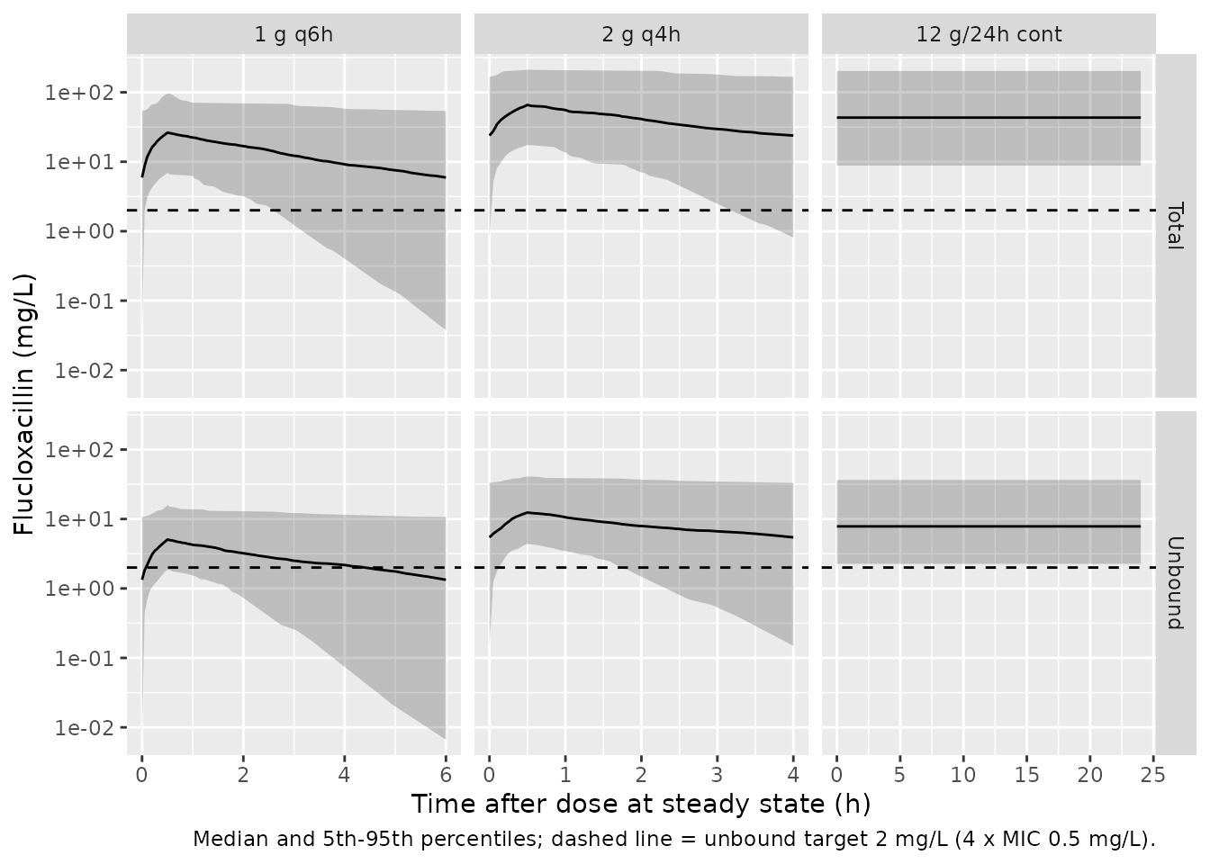
Probability of target attainment
The paper’s target is an unbound concentration above 4 x MIC for at
least 50% of the dosing interval (fT>4xMIC >= 50%), with MIC 0.5
mg/L, the cloxacillin ECOFF for MSSA. fT is the fraction of
the steady-state interval with the unbound concentration above the
threshold.
ft_above <- function(time, conc, thr) {
  # Fraction of the interval with conc > thr; each grid step is weighted by
  # its width, using the left end-point.
  dt <- diff(time)
  sum(dt * (head(conc, -1) > thr)) / sum(dt)
}

pta_subject <- sim_ss |>
  dplyr::group_by(regimen, id) |>
  dplyr::summarise(
    ft_mic = ft_above(time, Cu, 0.5),
    ft_4mic = ft_above(time, Cu, 2),
    cl = cl[1], fu = fu[1],
    .groups = "drop"
  )

paper_s3_final <- tibble::tribble(
  ~regimen,        ~paper_50_mic, ~paper_50_4mic, ~paper_100_mic, ~paper_100_4mic,
  "1 g q6h",                  23,              3,             11,               2,
  "1 g q4h",                  38,              8,             20,               4,
  "2 g q4h",                  53,             20,             30,              11,
  "6 g/24h cont",             51,              9,             51,               9,
  "12 g/24h cont",            76,             26,             76,              26,
  "18 g/24h cont",            86,             41,             86,              41,
  "24 g/24h cont",            90,             51,             90,              51
)

pta <- pta_subject |>
  dplyr::group_by(regimen) |>
  dplyr::summarise(
    sim_50_mic = 100 * mean(ft_mic >= 0.5),
    sim_50_4mic = 100 * mean(ft_4mic >= 0.5),
    sim_100_mic = 100 * mean(ft_mic >= 1),
    sim_100_4mic = 100 * mean(ft_4mic >= 1),
    .groups = "drop"
  ) |>
  dplyr::mutate(regimen = as.character(regimen)) |>
  dplyr::left_join(paper_s3_final, by = "regimen")

pta |>
  dplyr::select(regimen, sim_50_mic, paper_50_mic, sim_50_4mic, paper_50_4mic,
                sim_100_4mic, paper_100_4mic) |>
  dplyr::rename(
    "Regimen" = regimen,
    "50% fT>MIC, model" = sim_50_mic,
    "50% fT>MIC, Table S3" = paper_50_mic,
    "50% fT>4xMIC, model" = sim_50_4mic,
    "50% fT>4xMIC, Table S3" = paper_50_4mic,
    "100% fT>4xMIC, model" = sim_100_4mic,
    "100% fT>4xMIC, Table S3" = paper_100_4mic
  ) |>
knitr::kable(digits = 0, caption = "Probability of target attainment (%), MIC 0.5 mg/L: this model in the virtual cohort above against Table S3 (final model) of the paper.")| Regimen | 50% fT>MIC, model | 50% fT>MIC, Table S3 | 50% fT>4xMIC, model | 50% fT>4xMIC, Table S3 | 100% fT>4xMIC, model | 100% fT>4xMIC, Table S3 |
|---|---|---|---|---|---|---|
| 1 g q6h | 90 | 23 | 58 | 3 | 38 | 2 |
| 1 g q4h | 98 | 38 | 77 | 8 | 56 | 4 |
| 2 g q4h | 100 | 53 | 90 | 20 | 74 | 11 |
| 6 g/24h cont | 100 | 51 | 80 | 9 | 80 | 9 |
| 12 g/24h cont | 100 | 76 | 96 | 26 | 96 | 26 |
| 18 g/24h cont | 100 | 86 | 99 | 41 | 99 | 41 |
| 24 g/24h cont | 100 | 90 | 100 | 51 | 100 | 51 |
# Replicates Figure 2 of Meenks 2023: probability of fT>4xMIC >= 50% across
# MIC for each regimen.
mic_grid <- seq(0.0625, 4, by = 0.0625)
pta_curve <- sim_ss |>
  dplyr::group_by(regimen, id) |>
  dplyr::reframe(
    mic = mic_grid,
    ft = vapply(mic_grid, function(m) ft_above(time, Cu, 4 * m), numeric(1))
  ) |>
  dplyr::group_by(regimen, mic) |>
  dplyr::summarise(pta = 100 * mean(ft >= 0.5), .groups = "drop")

ggplot(pta_curve, aes(mic, pta, colour = regimen)) +
  geom_line() +
  geom_vline(xintercept = 0.5, linetype = "dashed") +
  geom_hline(yintercept = 90, linetype = "dotted") +
  labs(x = "MIC (mg/L)", y = "Probability of fT>4xMIC >= 50% (%)", colour = NULL,
       caption = "Replicates Figure 2 of Meenks 2023 with this model and the virtual cohort above.")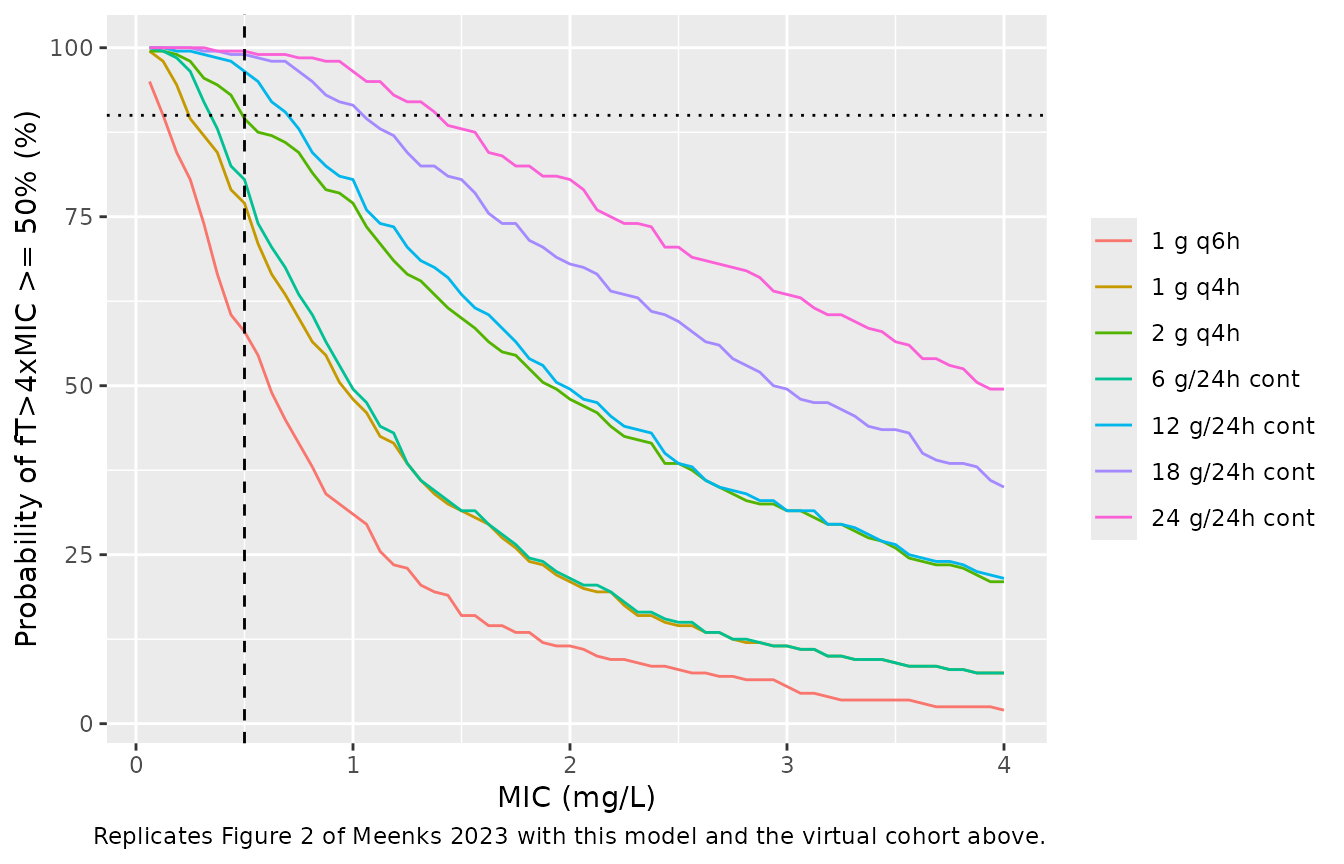
The model does not reproduce the paper’s final-model
attainment. For a continuous infusion the unbound steady state
is R / CL regardless of volume, albumin or fu,
so attainment depends only on the clearance distribution. With the
printed CL = fr * CLcr and the study’s CLcr distribution,
the median unbound clearance is about 64 L/h and the median unbound
steady state for 12 g/24 h about 7.8 mg/L, well above the 2 mg/L target.
Table S3’s 26% at 12 g/24 h and 51% at 24 g/24 h instead imply a median
unbound steady state near 1 mg/L at 12 g/24 h, that is a median unbound
clearance of roughly 480 L/h. Solving the printed
CL = fr * CLcr for that clearance needs a CLcr of about 425
mL/min/1.73 m^2. The same table’s MIC 0.5 mg/L rows (76% at 12 g/24 h)
give the same median, so this is not a single misprint.
# Continuous-infusion rows of Table S3 (final model): attainment = P(Css > thr).
# With a log-normal Css, P(Css > 2) and P(Css > 0.5) at the same rate fix
# both the median and the spread of Css.
z_4mic <- qnorm(0.26)
z_mic <- qnorm(0.76)
sd_log_css <- log(4) / (z_mic - z_4mic)
median_css <- exp(log(2) + z_4mic * sd_log_css)
data.frame(
  quantity = c("Median unbound Css at 12 g/24 h implied by Table S3 (mg/L)",
               "Implied median unbound CL (L/h)",
               "CLcr needed by CL = 19 * CLcr (mL/min/1.73 m^2)",
               "Median unbound CL in this model's cohort (L/h)"),
  value = c(median_css, 500 / median_css, 500 / median_css / (19 * 0.06),
            median(pta_subject$cl))
) |>
knitr::kable(digits = 2)| quantity | value |
|---|---|
| Median unbound Css at 12 g/24 h implied by Table S3 (mg/L) | 1.03 |
| Implied median unbound CL (L/h) | 484.09 |
| CLcr needed by CL = 19 * CLcr (mL/min/1.73 m^2) | 424.64 |
| Median unbound CL in this model’s cohort (L/h) | 63.82 |
Two readings of the structure were checked against the paper’s own output.
-
Clearance acting on total drug. If
fr * CLcrwere the clearance of total drug andCu = fu * Ctot, the unbound steady state would befu * R / CL. The attainment under that reading is shown below for the same cohort. It is closer to Table S3 but still above it. It is also inconsistent with the paper’s Figure 1, where most population-predicted concentrations of the (predominantly continuous-infusion, 12 g/24 h) cohort lie between 10 and 50 mg/L and reach 200 mg/L. Under the total-clearance reading the typical total steady state at 12 g/24 h and the mean CLcr is 6.7 mg/L. Under the unbound-clearance reading it is 30.6 mg/L, with 6.6 mg/L unbound. -
Clearance acting on unbound drug (implemented).
Additional file 1 states this reading explicitly. It also comes close to
the paper’s base-model attainment using the base-model
parameters alone (CL 52.8 L/h, 127% CV, no covariates). For a continuous
infusion that is
P(R / CL > thr)with log-normal CL, computed exactly in the second table below: it agrees within 2 points at 12-24 g/24 h and is 13 points higher at 6 g/24 h. Under the total-clearance reading the same base model would give about 55% at 12 g/24 h, against 92% in Table S3.
pta_subject |>
  dplyr::filter(grepl("cont", regimen)) |>
  dplyr::mutate(rate = as.numeric(sub(" g/24h cont", "", regimen)) * 1000 / 24) |>
  dplyr::group_by(regimen) |>
  dplyr::summarise(
    unbound_cl = 100 * mean(rate / cl > 2),
    total_cl = 100 * mean(fu * rate / cl > 2),
    .groups = "drop"
  ) |>
  dplyr::mutate(regimen = as.character(regimen)) |>
  dplyr::left_join(dplyr::select(paper_s3_final, regimen, paper_50_4mic), by = "regimen") |>
  dplyr::rename(
    "Regimen" = regimen,
    "CL on unbound drug (implemented)" = unbound_cl,
    "CL on total drug (alternative)" = total_cl,
    "Table S3 final model" = paper_50_4mic
  ) |>
knitr::kable(digits = 0, caption = "50% fT>4xMIC (%) for continuous infusion under the two readings.")| Regimen | CL on unbound drug (implemented) | CL on total drug (alternative) | Table S3 final model |
|---|---|---|---|
| 6 g/24h cont | 80 | 20 | 9 |
| 12 g/24h cont | 96 | 41 | 26 |
| 18 g/24h cont | 99 | 54 | 41 |
| 24 g/24h cont | 100 | 67 | 51 |
omega_base <- sqrt(log(1 + 1.27^2))
tibble::tibble(
  regimen = c("6 g/24h cont", "12 g/24h cont", "18 g/24h cont", "24 g/24h cont"),
  rate = c(6000, 12000, 18000, 24000) / 24,
  base_unbound_4mic = 100 * pnorm(log(rate / 2 / 52.8) / omega_base),
  base_unbound_mic = 100 * pnorm(log(rate / 0.5 / 52.8) / omega_base),
  paper_4mic = c(68, 92, 98, 99),
  paper_mic = c(99, 100, 100, 100)
) |>
  dplyr::select(regimen, base_unbound_4mic, paper_4mic, base_unbound_mic, paper_mic) |>
  dplyr::rename(
    "Regimen" = regimen,
    "50% fT>4xMIC, base model on unbound drug" = base_unbound_4mic,
    "50% fT>4xMIC, Table S3 base model" = paper_4mic,
    "50% fT>MIC, base model on unbound drug" = base_unbound_mic,
    "50% fT>MIC, Table S3 base model" = paper_mic
  ) |>
knitr::kable(digits = 0, caption = "Base model (Table 2 base-model column) attainment for continuous infusion, exact log-normal calculation, against Table S3.")| Regimen | 50% fT>4xMIC, base model on unbound drug | 50% fT>4xMIC, Table S3 base model | 50% fT>MIC, base model on unbound drug | 50% fT>MIC, Table S3 base model |
|---|---|---|---|---|
| 6 g/24h cont | 81 | 68 | 99 | 99 |
| 12 g/24h cont | 94 | 92 | 100 | 100 |
| 18 g/24h cont | 98 | 98 | 100 | 100 |
| 24 g/24h cont | 99 | 99 | 100 | 100 |
# Pins the documented discrepancy: under the printed final model the 12 g/24 h
# continuous-infusion attainment in a study-like cohort is far above the
# paper's 26%. The model-true value in this cohort is about 95%, so with
# n = 200 (binomial SE about 1.6 points) a 60% floor is over 20 SE away.
stopifnot(pta$sim_50_4mic[pta$regimen == "12 g/24h cont"] > 60)
The paper’s simulation cohort is not reported, so this difference cannot be explained from the article. It does not affect the fitted model, which is implemented as printed.
PKNCA validation
A single 2 g dose given as a 0.5 h infusion is simulated in 100
virtual patients with between-subject variability. For each subject the
unbound AUC0-inf must equal Dose / CL and the
total AUC0-inf must equal Dose / (CL * fu),
using the subject’s own CL and fu.
obs_nca <- c(0, 0.1, 0.25, 0.5, 0.6, 0.75, 1, 1.5, 2, 3, 4, 6, 8, 12, 16, 24,
             36, 48, 72, 96, 120, 168, 240)
cohort_nca <- make_cohort(100) |>
  dplyr::mutate(treatment = "2 g, 0.5 h infusion")
ev_nca <- cohort_nca |>
  dplyr::group_by(id) |>
  dplyr::reframe(
    time = c(0, obs_nca),
    evid = c(1L, rep(0L, length(obs_nca))),
    amt = c(2000, rep(NA_real_, length(obs_nca))),
    rate = c(4000, rep(0, length(obs_nca))),
    cmt = c("central", rep(NA_character_, length(obs_nca))),
    dvid = c(NA_integer_, rep(1L, length(obs_nca))),
    WT = WT[1], ALB = ALB[1], CRCL = CRCL[1], treatment = treatment[1]
  )

sim_nca <- rxode2::rxSolve(mod, ev_nca, sigma = NA, keep = "treatment",
                           rtol = 1e-10, atol = 1e-12, maxsteps = 1e6) |>
  as.data.frame()
stopifnot(!anyNA(sim_nca$Cu))
conc_nca <- sim_nca |>
  dplyr::select(id, time, treatment, Cu, Cc) |>
  tidyr::pivot_longer(c(Cu, Cc), names_to = "analyte", values_to = "conc") |>
  dplyr::filter(!is.na(conc))
stopifnot(all(conc_nca$conc >= -1e-6 * max(conc_nca$conc)))
conc_nca <- conc_nca |>
  dplyr::mutate(conc = pmax(conc, 0))

dose_nca <- ev_nca |>
  dplyr::filter(evid == 1) |>
  dplyr::select(id, time, treatment, amt)

conc_obj <- PKNCA::PKNCAconc(conc_nca, conc ~ time | treatment + id / analyte)
dose_obj <- PKNCA::PKNCAdose(dose_nca, amt ~ time | treatment + id,
                             route = "intravascular", duration = 0.5)
intervals <- data.frame(start = 0, end = Inf, cmax = TRUE, tmax = TRUE,
                        aucinf.obs = TRUE, half.life = TRUE)
nca_res <- PKNCA::pk.nca(PKNCA::PKNCAdata(conc_obj, dose_obj, intervals = intervals))

nca_wide <- as.data.frame(nca_res$result) |>
  dplyr::filter(PPTESTCD %in% c("cmax", "aucinf.obs", "half.life")) |>
  dplyr::select(id, analyte, PPTESTCD, PPORRES) |>
  tidyr::pivot_wider(names_from = PPTESTCD, values_from = PPORRES)

indiv <- sim_nca |>
  dplyr::distinct(id, cl, fu, vc)
nca_chk <- nca_wide |>
  dplyr::left_join(indiv, by = "id") |>
  dplyr::mutate(
    auc_closed = ifelse(analyte == "Cu", 2000 / cl, 2000 / (cl * fu)),
    pct_diff = 100 * (aucinf.obs / auc_closed - 1),
    thalf_closed = log(2) * vc / cl
  )

nca_chk |>
  dplyr::group_by(analyte) |>
  dplyr::summarise(
    cmax = median(cmax), aucinf = median(aucinf.obs), half_life = median(half.life),
    median_abs_pct_diff = median(abs(pct_diff)),
    .groups = "drop"
  ) |>
  dplyr::mutate(analyte = dplyr::recode(analyte, Cu = "Unbound", Cc = "Total")) |>
  dplyr::rename(
    "Analyte" = analyte,
    "Cmax (mg/L), median" = cmax,
    "AUC0-inf (mg*h/L), median" = aucinf,
    "t1/2 (h), median" = half_life,
    "Median |AUC0-inf - closed form| (%)" = median_abs_pct_diff
  ) |>
knitr::kable(digits = 2, caption = "PKNCA results after a single 2 g 0.5 h infusion, against each subject's closed-form AUC.")| Analyte | Cmax (mg/L), median | AUC0-inf (mg*h/L), median | t1/2 (h), median | Median |AUC0-inf - closed form| (%) |
|---|---|---|---|---|
| Total | 23.29 | 143.61 | 3.85 | 0.01 |
| Unbound | 4.38 | 27.60 | 3.85 | 0.01 |
stopifnot(
  # Structural: a wrong CLcr unit conversion or a fu applied the wrong way
  # moves every subject by tens of percent or more.
  abs(median(nca_chk$pct_diff)) < 1,
  # Envelope: trapezoid and terminal-slope error on the sampling grid.
  quantile(abs(nca_chk$pct_diff), 0.9) < 3,
  # One-compartment terminal half-life is log(2) * V / CL.
  quantile(abs(nca_chk$half.life / nca_chk$thalf_closed - 1), 0.9) < 0.02
)
The paper reports no NCA results, so there is no published table to compare against.
Assumptions and deviations
-
Typical unbound fraction 0.217, not 25%. The
printed covariate equation is
fu = 0.217 * (Alb / 21.2)^-exand the Results restate “The population estimate of the unbound fraction was 0.217”, while Table 2 listsfu= 25% (RSE 4.7%) for the final model. The equation value is used. One consistent explanation is that the iterative two-stage output in Table 2 is the arithmetic mean of the individual fu values, which sits above the typical value once IIV on fu and on the albumin exponent and the spread of albumin are included. Using 25% instead would lower every typical total concentration by about 13% (0.217 / 0.25) and leave unbound concentrations unchanged. -
Population means carried as typical values. Table 2
reports “Estimate, mean” with an IIV in %CV, and parameters were assumed
log-normal. The mean is used as the typical value and
omega^2 = log(1 + CV^2), as for the other MwPharm/EDSIM-built models in nlmixr2lib (Daskapan 2019, Geers 2022). If the printed means are instead arithmetic means of log-normal distributions, the typical values would be lower by a factor ofsqrt(1 + CV^2): 19 -> 15.5 for fr and 330 -> 253 L for V. -
No weight scaling on clearance. Additional file 1
says clearance was calculated “in L/h/70 kg^0.75”, but the final-model
clearance is
CL = fr * CLcrwith no weight term, and Table 2 givesfras the unitless ratio CL/CLcr. The printed equation is used. The typical clearance at the mean CLcr (75.2 L/h) matches the 77.5 L/h median quoted in the Discussion. - CLcr as printed. CLcr is the CKD-EPI estimate in mL/min/1.73 m^2 (Table 1), used without body-surface-area de-normalisation, which the paper does not describe.
- The Monte Carlo cohort is not reported. The virtual cohort in this article is drawn from the study’s demographics. The paper’s final-model target attainment (Table S3, Figure 2) is not reproduced, as shown in the target-attainment section. The base-model rows are reproduced from the base-model parameters, which supports the unbound-clearance structure.
- Unbound fraction is not capped. The equation can in principle exceed 1 at very low albumin combined with extreme random effects. The paper applies no bound, so none is added. At 10 g/L, the lowest albumin in Table S1, the typical fu is 0.36.
- Residual error. Proportional error on each endpoint as stated in Additional file 1. The %CV values of Table 2 are used directly as proportional SDs.
- Model performance. The paper reports a final-model bias of -27.1% and a precision of 53.3% (Results). Users should treat individual predictions accordingly.