Model and source
- Citation: Taneja A, Desrivot J, Diderichsen PM, Blanque R, Allamasey L, Fagard L, Fieuw A, Van der Aar E, Namour F. Population Pharmacokinetic and Pharmacodynamic Analysis of GLPG1690, an Autotaxin Inhibitor, in Healthy Volunteers and Patients with Idiopathic Pulmonary Fibrosis. Clin Pharmacokinet. 2019;58(9):1175-1188. doi:10.1007/s40262-019-00755-3
- Description: Two-compartment population PK with first-order absorption and dose-dependent apparent clearance, coupled to an effect-compartment Imax model for plasma lysophosphatidic acid (LPA) C18:2 reduction, for the autotaxin inhibitor GLPG1690 (ziritaxestat) in healthy volunteers and patients with idiopathic pulmonary fibrosis
- Article: https://doi.org/10.1007/s40262-019-00755-3 (open access, PMC6719325)
GLPG1690 (ziritaxestat) is an oral inhibitor of autotaxin, the enzyme that produces lysophosphatidic acid (LPA). Taneja 2019 fitted one combined population PK and PK/PD model to three studies. GLPG1690 plasma concentrations follow a two-compartment model with first-order absorption, and apparent clearance falls linearly with the total daily dose. The PD endpoint is plasma LPA C18:2, the most abundant plasma LPA species. It is described by an Imax model driven by an “effective concentration”: the plasma concentration plus a weighted effect-compartment concentration, which gives an immediate response and a delayed one.
Population
The pooled dataset (Taneja 2019 Table 1 and Table 2) combines:
- First-in-human study NCT02179502 (Belgium). Healthy male volunteers aged 18-50 years. In the single-ascending-dose (SAD) part, 16 volunteers received 20-1500 mg as an oral suspension or 300 mg as a capsule, over up to three occasions. In the multiple-ascending-dose (MAD) part, 24 volunteers took 150 mg twice daily, or 600 or 1000 mg once daily, as a suspension for 14 days (6 active and 2 placebo per cohort).
- Drug-drug interaction study IND130687 (USA). 18 healthy male volunteers received one 600 mg capsule before and after 10 days of rifampicin 600 mg once daily.
- Proof-of-concept study NCT02738801 (14 sites). 23 patients with idiopathic pulmonary fibrosis (IPF) aged 52-79 years were randomised to placebo (6) or 600 mg once daily as a capsule (17) for 12 weeks. This is the only study that enrolled women (43.75% of the analysed subjects).
Across studies, median body weight was 80.1-83.8 kg (range 64.2-110) and median BMI 24.5-29.7 kg/m^2. The analysis used 1348 GLPG1690 concentrations. Of the 1514 records, 166 (11%) were below the 1.00 ng/mL limit of quantification and were excluded. Each SAD occasion was entered as an independent subject, so the SAD part contributes 48 NONMEM IDs from 16 volunteers. Median baseline LPA C18:2 (the peak-area ratio to the LPA C17:0 internal standard) was 0.474 in the SAD part, 0.174 in the MAD part and 0.329 in the proof-of-concept study.
The same information is available programmatically via the model’s
population metadata
(readModelDb("Taneja_2019_glpg1690")()$population).
Source trace
The per-parameter origin is recorded as an in-file comment next to
each ini() entry in
inst/modeldb/specificDrugs/Taneja_2019_glpg1690.R. The
table below collects them in one place for review. Table 3 of the paper
gives every estimate on its estimation scale: footnote a =
log-transformed, b = probit, c = power covariate on a log-transformed
parameter, d = linear covariate on a probit-transformed parameter.
| Equation / parameter | Value | Source location |
|---|---|---|
lcl (CL/F) |
3.15 (23.3 L/h) | Table 3, CL |
lvc (VP2/F) |
2.65 (14.1 L) | Table 3, VP2 |
lka (KA) |
-1.51 (0.222 1/h) | Table 3, KA |
lq (Q23/F) |
0.130 (1.14 L/h) | Table 3, Q23 |
lvp (VP3/F) |
2.53 (12.5 L) | Table 3, VP3 |
probitimax (Imax) |
1.33 (90.8%) | Table 3, Imax (footnote b) |
lic50 (IC50) |
4.74 (114 ng/mL) | Table 3, IC50 |
lke0 (KEO) |
-2.32 (0.0982 1/h) | Table 3, KEO |
lcprel (CPREL) |
-1.20 (0.301; printed 0.303) | Table 3, CP REL |
e_dose_glpg1690_mgd_cl |
0.000415 per mg/day | Table 3, CL(DOSE) |
e_dis_ipf_vc |
5.59 (+559%) | Table 3, VP2 in IPF patients |
e_form_capsule_ka |
0.162 (+16.2%) | Table 3, KA (capsule) |
e_conmed_rifampicin_ka |
1.17 (+117%) | Table 3, KA with DDI |
e_conmed_rifampicin_fdepot |
-2.31 (F = 9.94%) | Table 3, Relative bioavailability F1 with DDI |
e_lpac182_bl_ic50 |
-0.473 | Table 3, IC50 (LPA C18:2 BL), footnote c |
e_lpac182_bl_imax |
0.5805 | Table 3, Imax (LPA C18:2 BL), footnote d |
e_occ2_imax |
-0.36 (83.33%) | Table 3, Imax at occasion 2 of the FIH study, SAD part |
e_occ3_imax |
-0.4504 (80.97%) | Table 3, Imax at occasion 3 of the FIH study, SAD part |
e_day14_imax |
0.2043 (93.72%) | Table 3, Imax at day 14 and later of the FIH study, MAD part |
e_dis_ipf_ruv |
0.209 (+23.3% variance) | Table 3, GLPG1690 RUV in patients with IPF |
e_dis_ipf_ruv_lpaC182 |
0.500 (+64.9% variance) | Table 3, Plasma LPA C18:2 RUV in patients with IPF |
etalcl, etalvc block |
0.294, 0.357, 0.877 | Table 3, BSV variance column (correlation 70.3%) |
etalka |
0.0194 | Table 3, KA BSV variance |
etalic50 |
0.129 | Table 3, IC50 BSV variance |
etaprobitimax |
0.0324 | Table 3, Imax BSV variance |
expSd |
sqrt(0.200) = 0.447 | Table 3, GLPG1690 RUV (44.8%cv) |
expSd_lpaC182 |
sqrt(0.0762) = 0.276 | Table 3, Plasma LPA C18:2 RUV (27.6%cv) |
| Absorption, central and peripheral ODEs | n/a | Sect. 3.2 display equations; Fig. 3 |
d/dt(effect) <- ke0 * (Cc - effect) |
n/a | Sect. 3.2, dCpe/dt = KEO (Cplasma - Cpe) |
cl = TVCL * (1 - CLSLP * DOSE) |
n/a | Sect. 3.2 and Fig. 3 |
ceff = Cc + cprel * effect |
n/a | Sect. 3.2, CEFF = Cplasma + CPREL Cpe |
lpaC182 = LPAC182_BL * (1 - imax * ceff / (ceff + ic50)) |
n/a | Sect. 3.2 and Fig. 3 |
| Log-transformed data, additive error; IPF effect on the RUV variance | n/a | Sect. 3.2, paragraph after Table 3 |
| Typical baseline LPA C18:2 = 0.36 (covariate centring) | n/a | Sect. 2.3.9; Sect. 3.3 (“For an LPA C18:2 BL of 0.36 … 91%”) |
Covariate back-transforms
Table 3 prints each covariate effect twice: as the estimate on the
estimation scale, and as a physical-units summary (for example “83.33%”
for Imax on the second SAD occasion). The chunk below reads the
individual imax and ic50 back from the solved
model for each covariate pattern, and checks them against those printed
summaries. It does not recompute the equations separately. The model and
the check use the same parameters, so the only difference is the
rounding of the printed values.
mod <- readModelDb("Taneja_2019_glpg1690")

patterns <- tibble::tribble(
  ~pattern, ~LPAC182_BL, ~OCC, ~STUDY_FIH_MAD, ~DAY14, ~published_imax_pct,
  "Typical, baseline 0.36", 0.36, 0, 0, 0, 90.8,
  "Baseline 0.36 + 0.1", 0.46, 0, 0, 0, 91.7,
  "SAD occasion 2", 0.36, 2, 0, 0, 83.33,
  "SAD occasion 3", 0.36, 3, 0, 0, 80.97,
  "MAD part, day 14 and later", 0.36, 0, 1, 1, 93.72,
  "Proof-of-concept study past day 14", 0.36, 0, 0, 1, 90.8
)

bt_events <- patterns |>
  dplyr::mutate(
    id = dplyr::row_number(),
    time = 1,
    evid = 0L,
    amt = 0,
    cmt = NA_character_,
    dvid = 1L,
    DOSE_GLPG1690_MGD = 600,
    FORM_CAPSULE = 1,
    CONMED_RIFAMPICIN = 0,
    DIS_IPF = 1
  ) |>
  dplyr::relocate(id, time, evid, amt, cmt, dvid)

bt <- rxode2::rxSolve(
  mod,
  events = bt_events,
  omega = NA,
  sigma = NA,
  keep = "pattern",
  returnType = "data.frame"
) |>
  dplyr::select(pattern, imax, ic50) |>
  dplyr::left_join(patterns |> dplyr::select(pattern, published_imax_pct), by = "pattern") |>
  dplyr::mutate(model_imax_pct = 100 * imax)
#> ℹ parameter labels from comments will be replaced by 'label()'

bt |>
  dplyr::select(pattern, published_imax_pct, model_imax_pct, ic50) |>
  dplyr::rename(
    "Covariate pattern" = pattern,
    "Imax, Table 3 (%)" = published_imax_pct,
    "Imax, model (%)" = model_imax_pct,
    "IC50, model (ng/mL)" = ic50
  ) |>
knitr::kable(digits = 2, caption = "Imax and IC50 by covariate pattern.")| Covariate pattern | Imax, Table 3 (%) | Imax, model (%) | IC50, model (ng/mL) |
|---|---|---|---|
| Typical, baseline 0.36 | 90.80 | 90.82 | 114.43 |
| Baseline 0.36 + 0.1 | 91.70 | 91.74 | 101.91 |
| SAD occasion 2 | 83.33 | 83.40 | 114.43 |
| SAD occasion 3 | 80.97 | 81.05 | 114.43 |
| MAD part, day 14 and later | 93.72 | 93.75 | 114.43 |
| Proof-of-concept study past day 14 | 90.80 | 90.82 | 114.43 |
ic50_ratio <- bt$ic50[bt$pattern == "Baseline 0.36 + 0.1"] /
  bt$ic50[bt$pattern == "Typical, baseline 0.36"]

stopifnot(
  nrow(bt) == nrow(patterns),
  # Printed to 1-2 decimals; the largest rounding residual is 0.08 points
  # (occasion 3: pnorm(0.8796) = 81.05 vs printed 80.97).
  all(abs(bt$model_imax_pct - bt$published_imax_pct) < 0.15),
  abs(bt$ic50[bt$pattern == "Typical, baseline 0.36"] - 114) < 0.5
)
Raising baseline LPA C18:2 by 0.1 changes IC50 by -10.95%. This is
not the “-4.41% change/+10%” printed in Table 3: that figure is the
change for a 10% relative increase in baseline,
1.1^-0.473 - 1 = -4.41%. At the typical baseline of 0.36,
+0.1 is +28%, which gives (0.46 / 0.36)^-0.473 - 1. The
12-week proof-of-concept study also samples past day 14, but the day-14
effect is gated to the MAD part through STUDY_FIH_MAD, so
that row keeps the typical Imax.
Typical-patient steady state (Table 4)
Taneja 2019 Sect. 2.3.9 defines the default simulation scenario: a
typical patient with IPF (DIS_IPF = 1), taking capsules
(FORM_CAPSULE = 1), without rifampicin, with a baseline LPA
C18:2 of 0.36 and all random effects at zero. Table 4 reports
steady-state Cmax, AUC over 24 h, maximal LPA C18:2 reduction and the
24-h area under the percent-reduction curve (AUEC). These are given for
total daily doses of 50-1000 mg, taken once (QD) or twice (BID) daily.
The simulation below doses for 20 days and summarises the final 24 h
(day 20).
tau_start <- 19 * 24

make_regimen <- function(id, daily, reg, ndays = 20) {
  n_per_day <- if (reg == "BID") 2L else 1L
  ii <- 24 / n_per_day
  doses <- tibble::tibble(
    id = id,
    time = seq(0, by = ii, length.out = ndays * n_per_day),
    evid = 1L,
    amt = daily / n_per_day,
    cmt = "depot",
    dvid = NA_integer_
  )
  obs <- tibble::tibble(
    id = id,
    time = sort(unique(c(seq(0, tau_start, by = 24), tau_start + seq(0, 24, by = 0.05)))),
    evid = 0L,
    amt = 0,
    cmt = NA_character_,
    dvid = 1L
  )
  dplyr::bind_rows(doses, obs) |>
    dplyr::arrange(time, dplyr::desc(evid)) |>
    dplyr::mutate(
      regimen = paste(daily, reg),
      DOSE_GLPG1690_MGD = daily,
      FORM_CAPSULE = 1,
      CONMED_RIFAMPICIN = 0,
      DIS_IPF = 1,
      LPAC182_BL = 0.36,
      OCC = 0,
      STUDY_FIH_MAD = 0,
      DAY14 = 0
    )
}

table4_grid <- tidyr::expand_grid(
  daily = c(50, 100, 150, 200, 300, 600, 1000),
  reg = c("QD", "BID")
)
regimen_levels <- paste(table4_grid$daily, table4_grid$reg)

typ_events <- dplyr::bind_rows(lapply(seq_len(nrow(table4_grid)), function(i) {
  make_regimen(i, table4_grid$daily[i], table4_grid$reg[i])
})) |>
  dplyr::relocate(id, time, evid, amt, cmt, dvid)
stopifnot(!anyDuplicated(unique(typ_events[, c("id", "time", "evid")])))
# Tight tolerances: the closed-form AUC gate below compares this solve with
# DailyDose / CL(DailyDose), which uses the same parameters.
sim_typ <- rxode2::rxSolve(
  mod,
  events = typ_events,
  omega = NA,
  sigma = NA,
  keep = "regimen",
  returnType = "data.frame",
  rtol = 1e-10,
  atol = 1e-12
) |>
  dplyr::mutate(
    regimen = factor(regimen, levels = regimen_levels),
    lpa_red_pct = 100 * (1 - lpaC182 / LPAC182_BL)
  )
# Replicates the typical-patient profiles behind Taneja 2019 Table 4.
sim_typ |>
  dplyr::filter(time >= tau_start, grepl("^(200|600|1000) ", regimen)) |>
  dplyr::mutate(tad = time - tau_start) |>
  tidyr::pivot_longer(c(Cc, lpa_red_pct), names_to = "quantity", values_to = "value") |>
  dplyr::mutate(quantity = dplyr::recode(
    quantity,
    Cc = "GLPG1690 (ng/mL)",
    lpa_red_pct = "LPA C18:2 reduction (%)"
  )) |>
  ggplot(aes(tad, value, colour = regimen)) +
  geom_line() +
  facet_wrap(~quantity, scales = "free_y") +
  labs(
    x = "Time after the day-20 morning dose (h)",
    y = NULL,
    colour = "Total daily dose (mg)",
    title = "Typical IPF patient at steady state",
    caption = "Typical-value simulation for the Table 4 scenario of Taneja 2019."
  )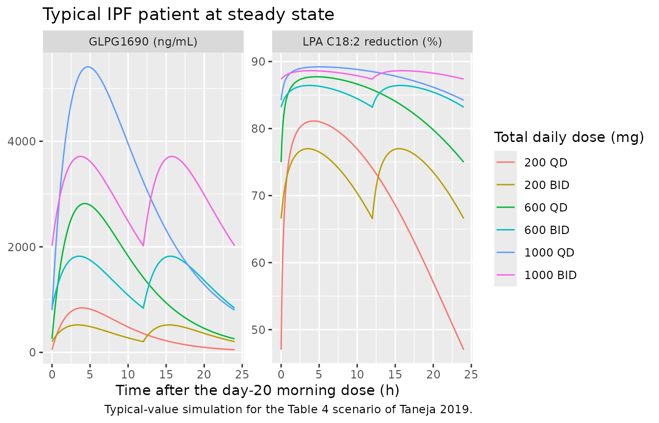
PKNCA computes Cmax and AUC0-24 over the day-20 dosing interval for the PK. The same machinery computes the maximum and the 24-h area of the percent LPA C18:2 reduction for the PD.
typ_conc <- sim_typ |>
  dplyr::filter(!is.na(Cc)) |>
  dplyr::select(id, time, Cc, lpa_red_pct, regimen)

typ_dose <- typ_events |>
  dplyr::filter(evid == 1) |>
  dplyr::select(id, time, amt, regimen) |>
  dplyr::mutate(regimen = factor(regimen, levels = regimen_levels))

ss_interval <- data.frame(
  start = tau_start,
  end = tau_start + 24,
  cmax = TRUE,
  auclast = TRUE
)

nca_pk <- PKNCA::pk.nca(PKNCA::PKNCAdata(
  PKNCA::PKNCAconc(typ_conc, Cc ~ time | regimen + id),
  PKNCA::PKNCAdose(typ_dose, amt ~ time | regimen + id),
  intervals = ss_interval
))

nca_pd <- PKNCA::pk.nca(PKNCA::PKNCAdata(
  PKNCA::PKNCAconc(typ_conc, lpa_red_pct ~ time | regimen + id),
  PKNCA::PKNCAdose(typ_dose, amt ~ time | regimen + id),
  intervals = ss_interval
))
table4 <- tibble::tribble(
  ~regimen, ~cmax, ~auc_ugh, ~maxred, ~auec,
  "50 QD", 204, 2.19, 60.7, 1010,
  "50 BID", 124, 2.19, 51.8, 1100,
  "100 QD", 413, 4.48, 73, 1360,
  "100 BID", 252, 4.48, 66.3, 1470,
  "150 QD", 626, 6.86, 78.2, 1550,
  "150 BID", 385, 6.86, 73.1, 1650,
  "200 QD", 845, 9.36, 81.1, 1670,
  "200 BID", 522, 9.36, 77, 1770,
  "300 QD", 1300, 14.7, 84.3, 1820,
  "300 BID", 811, 14.7, 81.4, 1900,
  "600 QD", 2830, 34.3, 87.7, 2020,
  "600 BID", 1830, 34.3, 86.4, 2050,
  "1000 QD", 5420, 73.3, 89.2, 2110,
  "1000 BID", 3720, 73.3, 88.6, 2120
) |>
  dplyr::mutate(regimen = factor(regimen, levels = regimen_levels))

# PK: ng/mL and ng*h/mL (Table 4 prints AUC in ug*h/mL).
cmp_pk <- nlmixr2lib::ncaComparisonTable(
  simulated = nca_pk,
  reference = table4 |>
    dplyr::transmute(regimen, cmax, auclast = 1000 * auc_ugh),
  by = "regimen",
  units = c(cmax = "ng/mL", auclast = "ng*h/mL, 0-24 h"),
  tolerance_pct = 20
)
knitr::kable(
  cmp_pk,
  caption = paste(
    "Steady-state GLPG1690 exposure in the typical IPF patient:",
    "simulated vs Taneja 2019 Table 4. * differs from reference by >20%."
  )
)| NCA parameter | regimen | Reference | Simulated | % diff |
|---|---|---|---|---|
| Cmax (ng/mL) | 50 QD | 204 | 203 | -0.3% |
| Cmax (ng/mL) | 50 BID | 124 | 124 | -0.1% |
| Cmax (ng/mL) | 100 QD | 413 | 412 | -0.3% |
| Cmax (ng/mL) | 100 BID | 252 | 252 | -0.1% |
| Cmax (ng/mL) | 150 QD | 626 | 625 | -0.2% |
| Cmax (ng/mL) | 150 BID | 385 | 384 | -0.3% |
| Cmax (ng/mL) | 200 QD | 845 | 843 | -0.2% |
| Cmax (ng/mL) | 200 BID | 522 | 521 | -0.2% |
| Cmax (ng/mL) | 300 QD | 1300 | 1300 | -0.2% |
| Cmax (ng/mL) | 300 BID | 811 | 809 | -0.2% |
| Cmax (ng/mL) | 600 QD | 2830 | 2820 | -0.3% |
| Cmax (ng/mL) | 600 BID | 1830 | 1820 | -0.4% |
| Cmax (ng/mL) | 1000 QD | 5420 | 5410 | -0.2% |
| Cmax (ng/mL) | 1000 BID | 3720 | 3710 | -0.2% |
| AUClast (ng*h/mL, 0-24 h) | 50 QD | 2190 | 2190 | -0.1% |
| AUClast (ng*h/mL, 0-24 h) | 50 BID | 2190 | 2190 | -0.1% |
| AUClast (ng*h/mL, 0-24 h) | 100 QD | 4480 | 4470 | -0.2% |
| AUClast (ng*h/mL, 0-24 h) | 100 BID | 4480 | 4470 | -0.2% |
| AUClast (ng*h/mL, 0-24 h) | 150 QD | 6860 | 6850 | -0.1% |
| AUClast (ng*h/mL, 0-24 h) | 150 BID | 6860 | 6850 | -0.1% |
| AUClast (ng*h/mL, 0-24 h) | 200 QD | 9360 | 9350 | -0.1% |
| AUClast (ng*h/mL, 0-24 h) | 200 BID | 9360 | 9350 | -0.1% |
| AUClast (ng*h/mL, 0-24 h) | 300 QD | 14700 | 14700 | -0.1% |
| AUClast (ng*h/mL, 0-24 h) | 300 BID | 14700 | 14700 | -0.1% |
| AUClast (ng*h/mL, 0-24 h) | 600 QD | 34300 | 34200 | -0.2% |
| AUClast (ng*h/mL, 0-24 h) | 600 BID | 34300 | 34200 | -0.2% |
| AUClast (ng*h/mL, 0-24 h) | 1000 QD | 73300 | 73300 | -0.1% |
| AUClast (ng*h/mL, 0-24 h) | 1000 BID | 73300 | 73300 | -0.1% |
pd_sim <- as.data.frame(nca_pd$result) |>
  dplyr::select(regimen, PPTESTCD, PPORRES) |>
  tidyr::pivot_wider(names_from = PPTESTCD, values_from = PPORRES) |>
  dplyr::mutate(regimen = factor(regimen, levels = regimen_levels))

cmp_pd <- table4 |>
  dplyr::select(regimen, maxred, auec) |>
  dplyr::left_join(pd_sim, by = "regimen") |>
  dplyr::mutate(
    maxred_diff = cmax - maxred,
    auec_pct = 100 * (auclast / auec - 1)
  )
stopifnot(nrow(cmp_pd) == 14, !anyNA(cmp_pd$cmax), !anyNA(cmp_pd$auclast))

cmp_pd |>
  dplyr::select(regimen, maxred, cmax, maxred_diff, auec, auclast, auec_pct) |>
  dplyr::rename(
    "Regimen (mg/day)" = regimen,
    "Max reduction, Table 4 (%)" = maxred,
    "Max reduction, simulated (%)" = cmax,
    "Difference (points)" = maxred_diff,
    "AUEC, Table 4 (%h)" = auec,
    "AUEC, simulated (%h)" = auclast,
    "AUEC % diff" = auec_pct
  ) |>
  knitr::kable(
    digits = 1,
    caption = paste(
      "Steady-state LPA C18:2 reduction in the typical IPF patient:",
      "simulated vs Taneja 2019 Table 4."
    )
)| Regimen (mg/day) | Max reduction, Table 4 (%) | Max reduction, simulated (%) | Difference (points) | AUEC, Table 4 (%h) | AUEC, simulated (%h) | AUEC % diff |
|---|---|---|---|---|---|---|
| 50 QD | 60.7 | 60.6 | -0.1 | 1010 | 1011.2 | 0.1 |
| 50 BID | 51.8 | 51.7 | -0.1 | 1100 | 1096.1 | -0.4 |
| 100 QD | 73.0 | 72.9 | -0.1 | 1360 | 1358.9 | -0.1 |
| 100 BID | 66.3 | 66.2 | -0.1 | 1470 | 1465.3 | -0.3 |
| 150 QD | 78.2 | 78.2 | 0.0 | 1550 | 1549.2 | 0.0 |
| 150 BID | 73.1 | 73.0 | -0.1 | 1650 | 1652.5 | 0.2 |
| 200 QD | 81.1 | 81.1 | 0.0 | 1670 | 1672.1 | 0.1 |
| 200 BID | 77.0 | 77.0 | 0.0 | 1770 | 1766.0 | -0.2 |
| 300 QD | 84.3 | 84.3 | 0.0 | 1820 | 1823.3 | 0.2 |
| 300 BID | 81.4 | 81.4 | 0.0 | 1900 | 1897.0 | -0.2 |
| 600 QD | 87.7 | 87.7 | 0.0 | 2020 | 2015.8 | -0.2 |
| 600 BID | 86.4 | 86.4 | 0.0 | 2050 | 2049.6 | 0.0 |
| 1000 QD | 89.2 | 89.2 | 0.0 | 2110 | 2106.0 | -0.2 |
| 1000 BID | 88.6 | 88.6 | 0.0 | 2120 | 2117.6 | -0.1 |
pk_wide <- as.data.frame(nca_pk$result) |>
  dplyr::select(regimen, PPTESTCD, PPORRES) |>
  tidyr::pivot_wider(names_from = PPTESTCD, values_from = PPORRES) |>
  dplyr::mutate(regimen = factor(regimen, levels = regimen_levels)) |>
  dplyr::left_join(table4 |> dplyr::rename(cmax_pub = cmax), by = "regimen") |>
  dplyr::mutate(
    cmax_pct = 100 * (cmax / cmax_pub - 1),
    auc_pct = 100 * (auclast / (1000 * auc_ugh) - 1)
  )
stopifnot(nrow(pk_wide) == 14, !anyNA(pk_wide$cmax_pct), !anyNA(pk_wide$auc_pct))

# Deterministic, typical-value comparisons. Table 4 reports the median of 250
# parameter-uncertainty draws and rounds to 3 significant figures. Measured
# residuals: AUC <= 0.21%, Cmax <= 0.4%, maximal reduction <= 0.1 points,
# AUEC <= 0.4%. A mis-transcribed clearance slope, volume, ka or IC50 moves
# these by 10% or more.
stopifnot(
  max(abs(pk_wide$auc_pct)) < 1,
  max(abs(pk_wide$cmax_pct)) < 1.5,
  max(abs(cmp_pd$maxred_diff)) < 0.5,
  max(abs(cmp_pd$auec_pct)) < 1.5
)
Every regimen matches Table 4 closely. The AUCs agree to within 0.21%, the Cmax values to within 0.4%, the maximal LPA C18:2 reductions to within 0.1 percentage points, and the AUECs to within 0.4%. The paper’s values are medians over 250 parameter-uncertainty draws rather than a single typical-value solve, so small differences are expected.
Dose-dependent clearance: closed-form check
At steady state, the AUC over one day equals the daily dose divided
by the apparent clearance at that dose. Here that is
DailyDose / (23.3 * (1 - 0.000415 * DailyDose)), and F1 = 1
without rifampicin. The QD and BID regimens of the same daily dose must
therefore have the same AUC, as Table 4 shows. This check confirms that
the covariate is the total daily dose, not the amount
given per administration.
cf <- pk_wide |>
  dplyr::mutate(
    daily = as.numeric(sub(" .*", "", as.character(regimen))),
    auc_closed = 1000 * daily / (exp(3.15) * (1 - 0.000415 * daily)),
    rel_err = auclast / auc_closed - 1
  )
cf |>
  dplyr::select(regimen, auc_closed, auclast, rel_err) |>
  dplyr::mutate(rel_err = 100 * rel_err) |>
  dplyr::rename(
    "Regimen (mg/day)" = regimen,
    "Closed form (ng*h/mL)" = auc_closed,
    "PKNCA (ng*h/mL)" = auclast,
    "% diff" = rel_err
  ) |>
knitr::kable(digits = 3, caption = "Steady-state AUC0-24 vs DailyDose / CL(DailyDose).")| Regimen (mg/day) | Closed form (ng*h/mL) | PKNCA (ng*h/mL) | % diff |
|---|---|---|---|
| 50 QD | 2188.007 | 2187.973 | -0.002 |
| 50 BID | 2188.007 | 2187.975 | -0.001 |
| 100 QD | 4470.749 | 4470.680 | -0.002 |
| 100 BID | 4470.749 | 4470.684 | -0.001 |
| 150 QD | 6854.512 | 6854.410 | -0.001 |
| 150 BID | 6854.512 | 6854.415 | -0.001 |
| 200 QD | 9346.156 | 9346.020 | -0.001 |
| 200 BID | 9346.156 | 9346.026 | -0.001 |
| 300 QD | 14683.767 | 14683.562 | -0.001 |
| 300 BID | 14683.767 | 14683.573 | -0.001 |
| 600 QD | 34236.053 | 34235.646 | -0.001 |
| 600 BID | 34236.053 | 34235.668 | -0.001 |
| 1000 QD | 73251.499 | 73250.831 | -0.001 |
| 1000 BID | 73251.499 | 73250.868 | -0.001 |
Rifampicin: bioavailability, not clearance
Taneja 2019 found that rifampicin coadministration raises the
absorption rate by 117% and lowers relative bioavailability to 9.94%,
with no effect on clearance (Sect. 3.3 and Sect. 4). For a single 600 mg
capsule in a healthy volunteer, AUC0-inf with rifampicin divided by
AUC0-inf without it should therefore be exactly
exp(-2.31).
ddi_events <- tidyr::expand_grid(
  CONMED_RIFAMPICIN = c(0, 1),
  time = c(0, seq(0.1, 24, by = 0.1), seq(25, 400, by = 1))
) |>
  dplyr::mutate(
    id = CONMED_RIFAMPICIN + 1L,
    evid = 0L,
    amt = 0,
    cmt = NA_character_,
    dvid = 1L
  )
ddi_events <- dplyr::bind_rows(
  tibble::tibble(
    id = 1:2, time = 0, evid = 1L, amt = 600, cmt = "depot",
    dvid = NA_integer_, CONMED_RIFAMPICIN = c(0, 1)
  ),
  ddi_events
) |>
  dplyr::arrange(id, time, dplyr::desc(evid)) |>
  dplyr::mutate(
    arm = ifelse(CONMED_RIFAMPICIN == 1, "With rifampicin", "Without rifampicin"),
    DOSE_GLPG1690_MGD = 600,
    FORM_CAPSULE = 1,
    DIS_IPF = 0,
    LPAC182_BL = 0.36,
    OCC = 0,
    STUDY_FIH_MAD = 0,
    DAY14 = 0
  ) |>
  dplyr::relocate(id, time, evid, amt, cmt, dvid)

sim_ddi <- rxode2::rxSolve(
  mod,
  events = ddi_events,
  omega = NA,
  sigma = NA,
  keep = "arm",
  returnType = "data.frame",
  rtol = 1e-10,
  atol = 1e-12
)

nca_ddi <- PKNCA::pk.nca(PKNCA::PKNCAdata(
  PKNCA::PKNCAconc(sim_ddi |> dplyr::filter(!is.na(Cc)) |> dplyr::select(id, time, Cc, arm), Cc ~ time | arm + id),
  PKNCA::PKNCAdose(ddi_events |> dplyr::filter(evid == 1) |> dplyr::select(id, time, amt, arm), amt ~ time | arm + id),
  intervals = data.frame(start = 0, end = Inf, cmax = TRUE, tmax = TRUE, aucinf.obs = TRUE)
))

ddi_tab <- as.data.frame(nca_ddi$result) |>
  dplyr::filter(PPTESTCD %in% c("cmax", "tmax", "aucinf.obs")) |>
  dplyr::select(arm, PPTESTCD, PPORRES) |>
  tidyr::pivot_wider(names_from = PPTESTCD, values_from = PPORRES)
ddi_tab |>
  dplyr::rename(
    "Arm" = arm,
    "Cmax (ng/mL)" = cmax,
    "Tmax (h)" = tmax,
    "AUC0-inf (ng*h/mL)" = aucinf.obs
  ) |>
knitr::kable(digits = 2, caption = "Typical healthy volunteer, single 600 mg capsule.")| Arm | Cmax (ng/mL) | Tmax (h) | AUC0-inf (ng*h/mL) |
|---|---|---|---|
| With rifampicin | 947.66 | 1.1 | 3396.03 |
| Without rifampicin | 5570.80 | 1.6 | 34226.14 |
auc_ratio <- ddi_tab$aucinf.obs[ddi_tab$arm == "With rifampicin"] /
  ddi_tab$aucinf.obs[ddi_tab$arm == "Without rifampicin"]
# The integrand is 10-fold smaller with rifampicin but decays at the same
# rate, so the ratio is exp(-2.31) up to trapezoid and extrapolation error
# (measured 0.04%).
stopifnot(length(auc_ratio) == 1, abs(auc_ratio / exp(-2.31) - 1) < 0.004)
The simulated AUC ratio is 0.09922, against exp(-2.31) =
0.09926. The paper did not publish NCA results for this study, so the
check confirms how the effect is encoded rather than reproducing a
published value.
Individual-patient simulations (Figure 7 and Table 5)
Sect. 2.3.9 describes the individual-patient simulations. Baseline LPA C18:2 is drawn from a uniform distribution over 0.14-0.59, the range of 15 of the proof-of-concept patients (one outlier at 1.3 was excluded). Between-subject random effects are drawn from the final-model OMEGA. Seven once-daily dose levels from 50 to 1000 mg are simulated in the typical IPF-patient scenario. The paper used 10,000 virtual patients per dose. Here each dose has 200, and each dose is solved separately.
rxode2::rxSetSeed(20190406)
n_per_dose <- 200L
qd_doses <- c(50, 100, 150, 200, 300, 600, 1000)

make_indiv <- function(daily, id_offset) {
  base <- tibble::tibble(
    id = id_offset + seq_len(n_per_dose),
    LPAC182_BL = stats::runif(n_per_dose, 0.14, 0.59)
  )
  doses <- tidyr::expand_grid(id = base$id, time = seq(0, by = 24, length.out = 20)) |>
    dplyr::mutate(evid = 1L, amt = daily, cmt = "depot", dvid = NA_integer_)
  obs <- tidyr::expand_grid(id = base$id, time = tau_start + seq(0, 24, by = 0.25)) |>
    dplyr::mutate(evid = 0L, amt = 0, cmt = NA_character_, dvid = 1L)
  dplyr::bind_rows(doses, obs) |>
    dplyr::left_join(base, by = "id") |>
    dplyr::arrange(id, time, dplyr::desc(evid)) |>
    dplyr::mutate(
      dose_level = paste(daily, "mg QD"),
      DOSE_GLPG1690_MGD = daily,
      FORM_CAPSULE = 1,
      CONMED_RIFAMPICIN = 0,
      DIS_IPF = 1,
      OCC = 0,
      STUDY_FIH_MAD = 0,
      DAY14 = 0
    ) |>
    dplyr::relocate(id, time, evid, amt, cmt, dvid)
}

set.seed(20190406)
indiv_events <- lapply(seq_along(qd_doses), function(i) {
  make_indiv(qd_doses[i], id_offset = (i - 1L) * n_per_dose)
})
stopifnot(!anyDuplicated(unique(dplyr::bind_rows(indiv_events)[, c("id", "time", "evid")])))
# IPRED only (sigma = NA): the paper summarises individual predictions, not
# simulated observations with residual error.
sim_ind <- dplyr::bind_rows(lapply(indiv_events, function(ev) {
  rxode2::rxSolve(
    mod,
    events = ev,
    sigma = NA,
    keep = "dose_level",
    returnType = "data.frame",
    maxsteps = 1e6
  )
})) |>
  dplyr::mutate(
    dose_level = factor(dose_level, levels = paste(qd_doses, "mg QD")),
    lpa_red_pct = 100 * (1 - lpaC182 / LPAC182_BL)
  )
stopifnot(!anyNA(sim_ind$Cc), !anyNA(sim_ind$lpaC182))
ind_conc <- sim_ind |>
  dplyr::filter(!is.na(Cc)) |>
  dplyr::select(id, time, Cc, lpa_red_pct, dose_level)
ind_dose <- dplyr::bind_rows(indiv_events) |>
  dplyr::filter(evid == 1) |>
  dplyr::select(id, time, amt, dose_level) |>
  dplyr::mutate(dose_level = factor(dose_level, levels = levels(sim_ind$dose_level)))

ind_pk <- PKNCA::pk.nca(PKNCA::PKNCAdata(
  PKNCA::PKNCAconc(ind_conc, Cc ~ time | dose_level + id),
  PKNCA::PKNCAdose(ind_dose, amt ~ time | dose_level + id),
  intervals = ss_interval
))
ind_pd <- PKNCA::pk.nca(PKNCA::PKNCAdata(
  PKNCA::PKNCAconc(ind_conc, lpa_red_pct ~ time | dose_level + id),
  PKNCA::PKNCAdose(ind_dose, amt ~ time | dose_level + id),
  intervals = ss_interval
))

ind_metrics <- dplyr::bind_rows(
  as.data.frame(ind_pk$result) |>
    dplyr::mutate(metric = dplyr::recode(PPTESTCD, cmax = "Cmax (ng/mL)", auclast = "AUC0-24 (ng*h/mL)")),
  as.data.frame(ind_pd$result) |>
    dplyr::mutate(metric = dplyr::recode(PPTESTCD, cmax = "Maximal LPA C18:2 reduction (%)", auclast = "AUEC0-24 (%h)"))
) |>
  dplyr::select(id, dose_level, metric, PPORRES)
# Replicates Figure 7 of Taneja 2019: percentiles of individual steady-state
# exposure and response across the once-daily dose range.
ind_metrics |>
  dplyr::group_by(dose_level, metric) |>
  dplyr::summarise(
    P2.5 = stats::quantile(PPORRES, 0.025),
    P10 = stats::quantile(PPORRES, 0.10),
    P25 = stats::quantile(PPORRES, 0.25),
    P50 = stats::quantile(PPORRES, 0.50),
    .groups = "drop"
  ) |>
  tidyr::pivot_longer(P2.5:P50, names_to = "percentile", values_to = "value") |>
  dplyr::mutate(
    dose = as.numeric(sub(" .*", "", as.character(dose_level))),
    percentile = factor(percentile, levels = c("P50", "P25", "P10", "P2.5"))
  ) |>
  ggplot(aes(dose, value, colour = percentile)) +
  geom_line() +
  geom_point() +
  facet_wrap(~metric, scales = "free_y") +
  labs(
    x = "GLPG1690 once-daily dose (mg)",
    y = NULL,
    colour = "Percentile",
    title = "Figure 7 - individual steady-state exposure and response",
    caption = "Replicates Figure 7 of Taneja 2019 (200 virtual IPF patients per dose)."
  )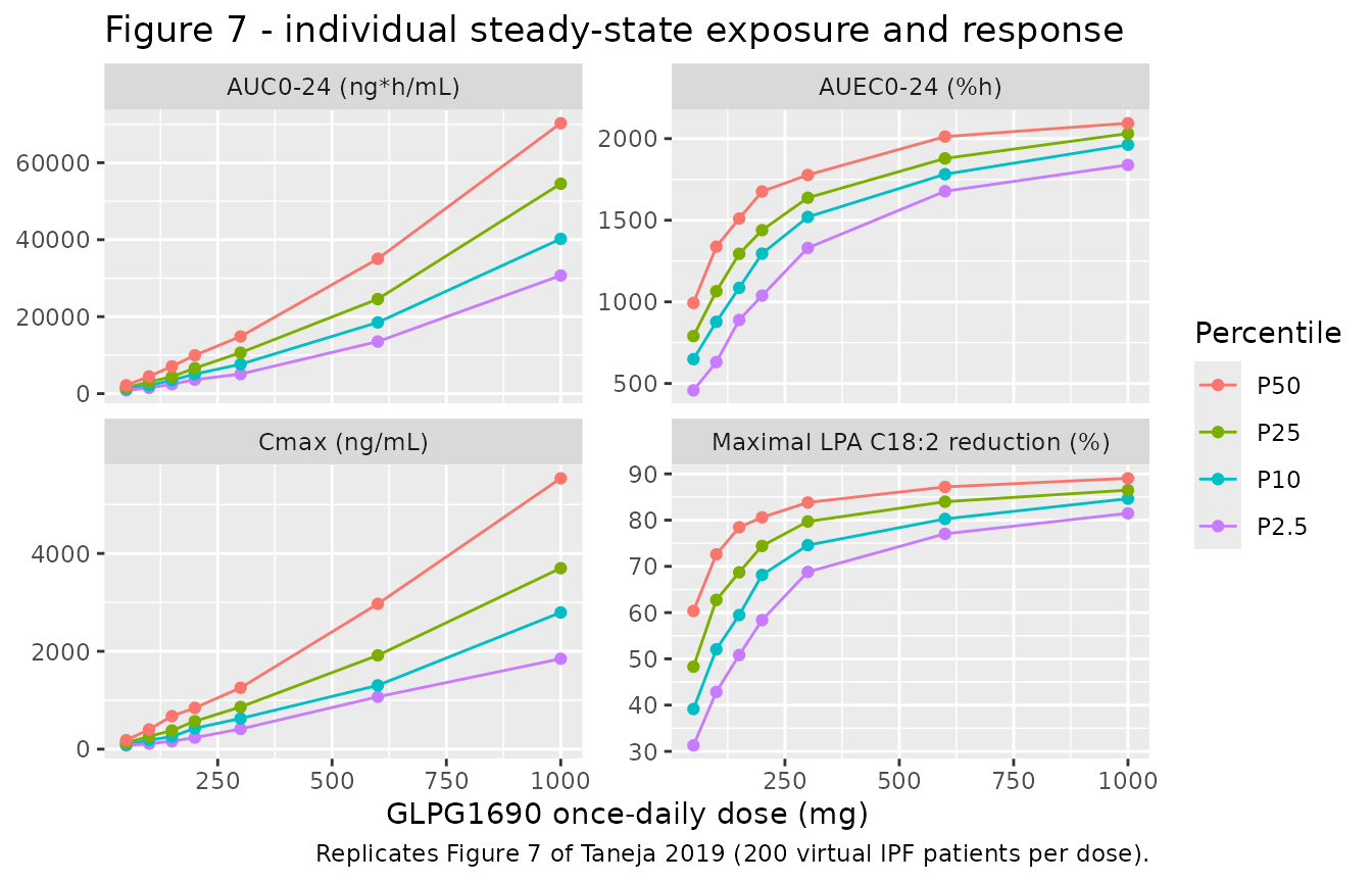
Table 5 summarises the individual simulations at 200, 300 and 600 mg once daily. The metrics are the percentage of patients whose maximal LPA C18:2 reduction reaches 50%, 80% or 90%, the percentage whose GLPG1690 concentration stays above IC50 for the whole dosing interval, and the median fraction of the interval spent above IC50, IC80 and IC90. The thresholds use the typical IC50 of 114 ng/mL (Sect. 3.4), with IC80 = 4 x IC50 and IC90 = 9 x IC50.
ic50_typ <- 114
tau_grid <- sim_ind |>
  dplyr::filter(time >= tau_start, time < tau_start + 24)

frac_above <- tau_grid |>
  dplyr::group_by(dose_level, id) |>
  dplyr::summarise(
    min_cc = min(Cc),
    f50 = mean(Cc > ic50_typ),
    f80 = mean(Cc > 4 * ic50_typ),
    f90 = mean(Cc > 9 * ic50_typ),
    .groups = "drop"
  )
maxred <- ind_metrics |>
  dplyr::filter(metric == "Maximal LPA C18:2 reduction (%)") |>
  dplyr::select(dose_level, id, maxred = PPORRES)

t5_sim <- frac_above |>
  dplyr::left_join(maxred, by = c("dose_level", "id")) |>
  dplyr::group_by(dose_level) |>
  dplyr::summarise(
    `Patients > IC50 for the entire dosing interval (%)` = 100 * mean(min_cc > ic50_typ),
    `Patients reaching 50% LPA C18:2 reduction (%)` = 100 * mean(maxred >= 50),
    `Patients reaching 80% LPA C18:2 reduction (%)` = 100 * mean(maxred >= 80),
    `Patients reaching 90% LPA C18:2 reduction (%)` = 100 * mean(maxred >= 90),
    `Median fraction of interval > IC50 (%)` = 100 * stats::median(f50),
    `Median fraction of interval > IC80 (%)` = 100 * stats::median(f80),
    `Median fraction of interval > IC90 (%)` = 100 * stats::median(f90),
    .groups = "drop"
  ) |>
  dplyr::filter(dose_level %in% c("200 mg QD", "300 mg QD", "600 mg QD")) |>
  tidyr::pivot_longer(-dose_level, names_to = "metric", values_to = "Simulated")

t5_pub <- tibble::tribble(
  ~metric, ~`200 mg QD`, ~`300 mg QD`, ~`600 mg QD`,
  "Patients > IC50 for the entire dosing interval (%)", 24.7, 43.4, 79.8,
  "Patients reaching 50% LPA C18:2 reduction (%)", 99.4, 99.9, 100,
  "Patients reaching 80% LPA C18:2 reduction (%)", 51.3, 69.7, 91.0,
  "Patients reaching 90% LPA C18:2 reduction (%)", 3.22, 7.39, 22.3,
  "Median fraction of interval > IC50 (%)", 79.0, 94.0, 100,
  "Median fraction of interval > IC80 (%)", 36.0, 51.0, 82.0,
  "Median fraction of interval > IC90 (%)", 0, 20.0, 54.0
) |>
  tidyr::pivot_longer(-metric, names_to = "dose_level", values_to = "Published")

t5 <- t5_pub |>
  dplyr::left_join(t5_sim |> dplyr::mutate(dose_level = as.character(dose_level)), by = c("metric", "dose_level")) |>
  dplyr::mutate(Difference = Simulated - Published)
stopifnot(nrow(t5) == 21, !anyNA(t5$Simulated))

t5 |>
  dplyr::rename("Summary variable" = metric, "Dose" = dose_level, "Table 5" = Published) |>
knitr::kable(digits = 1, caption = "Individual-patient steady-state summaries: simulated (200 per dose) vs Taneja 2019 Table 5.")| Summary variable | Dose | Table 5 | Simulated | Difference |
|---|---|---|---|---|
| Patients > IC50 for the entire dosing interval (%) | 200 mg QD | 24.7 | 27.0 | 2.3 |
| Patients > IC50 for the entire dosing interval (%) | 300 mg QD | 43.4 | 41.5 | -1.9 |
| Patients > IC50 for the entire dosing interval (%) | 600 mg QD | 79.8 | 83.0 | 3.2 |
| Patients reaching 50% LPA C18:2 reduction (%) | 200 mg QD | 99.4 | 100.0 | 0.6 |
| Patients reaching 50% LPA C18:2 reduction (%) | 300 mg QD | 99.9 | 100.0 | 0.1 |
| Patients reaching 50% LPA C18:2 reduction (%) | 600 mg QD | 100.0 | 100.0 | 0.0 |
| Patients reaching 80% LPA C18:2 reduction (%) | 200 mg QD | 51.3 | 52.5 | 1.2 |
| Patients reaching 80% LPA C18:2 reduction (%) | 300 mg QD | 69.7 | 73.0 | 3.3 |
| Patients reaching 80% LPA C18:2 reduction (%) | 600 mg QD | 91.0 | 91.0 | 0.0 |
| Patients reaching 90% LPA C18:2 reduction (%) | 200 mg QD | 3.2 | 6.5 | 3.3 |
| Patients reaching 90% LPA C18:2 reduction (%) | 300 mg QD | 7.4 | 8.0 | 0.6 |
| Patients reaching 90% LPA C18:2 reduction (%) | 600 mg QD | 22.3 | 23.0 | 0.7 |
| Median fraction of interval > IC50 (%) | 200 mg QD | 79.0 | 81.2 | 2.2 |
| Median fraction of interval > IC50 (%) | 300 mg QD | 94.0 | 93.2 | -0.8 |
| Median fraction of interval > IC50 (%) | 600 mg QD | 100.0 | 100.0 | 0.0 |
| Median fraction of interval > IC80 (%) | 200 mg QD | 36.0 | 38.5 | 2.5 |
| Median fraction of interval > IC80 (%) | 300 mg QD | 51.0 | 52.1 | 1.1 |
| Median fraction of interval > IC80 (%) | 600 mg QD | 82.0 | 84.4 | 2.4 |
| Median fraction of interval > IC90 (%) | 200 mg QD | 0.0 | 0.0 | 0.0 |
| Median fraction of interval > IC90 (%) | 300 mg QD | 20.0 | 22.9 | 2.9 |
| Median fraction of interval > IC90 (%) | 600 mg QD | 54.0 | 57.3 | 3.3 |
# Centre and envelope only: 200 subjects per dose gives a binomial standard
# error of up to 3.5 points on a proportion, and the thread-partitioned rxode2
# RNG draws a different cohort on every machine. Measured: every row within
# 3.3 points, median |difference| 1.2. The envelope of 12 points is over 3
# binomial SE; a mis-transcribed IC50, Imax or clearance slope moves these
# rows by 20 points or more.
stopifnot(
  stats::median(abs(t5$Difference)) < 5,
  max(abs(t5$Difference)) < 12
)

# Median individual AUC0-24 is close to the typical-value AUC, because the
# etas are log-normal with median 1 (Table 4: 9.36 / 14.7 / 34.3 ug*h/mL).
# The sampling SE of the log-median over 200 subjects is about 5%.
med_auc <- ind_metrics |>
  dplyr::filter(metric == "AUC0-24 (ng*h/mL)", dose_level %in% c("200 mg QD", "300 mg QD", "600 mg QD")) |>
  dplyr::group_by(dose_level) |>
  dplyr::summarise(med = stats::median(PPORRES), .groups = "drop") |>
  dplyr::mutate(ref = c(9360, 14700, 34300)[match(as.character(dose_level), c("200 mg QD", "300 mg QD", "600 mg QD"))])
stopifnot(nrow(med_auc) == 3, all(abs(med_auc$med / med_auc$ref - 1) < 0.2))
Every row of Table 5 is reproduced to within a few percentage points, which is the binomial noise expected from 200 patients per dose. This includes the interval-above-threshold rows. Their agreement is consistent with the paper having compared the plasma GLPG1690 concentration against the fixed typical IC50 of 114 ng/mL rather than against each patient’s own IC50.
Assumptions and deviations
-
Dose covariate is the total daily dose. Sect. 3.2
writes
CL_i(DOSE) = TVCL_i (1 - CLSLP DOSE)without saying whether DOSE is the amount per administration or per day. Table 4 prints the same AUC and the same 95% CI for the QD and BID rows of every daily dose. That is only possible if the two regimens share one clearance, soDOSE_GLPG1690_MGDis the total daily dose (the dose itself for single-dose records). The linear form reaches CL = 0 at about 2410 mg/day. Do not extrapolate beyond the studied maximum of 1500 mg/day. -
Effective concentration is a weighted sum. The Fig.
3 legend calls CPREL a “weighting factor between plasma and effect
compartment concentration”, but the printed equation is
CEFF = Cplasma + CPREL * Cpe. The equation is implemented as printed. - Centring of the baseline-LPA covariates. Table 3 does not print a reference value. Both relations are centred on 0.36, the typical baseline of the Sect. 2.3.9 simulations. This reproduces Sect. 3.3 (“For an LPA C18:2 BL of 0.36, the maximal reduction of LPA C18:2 was 91%”, i.e. pnorm(1.33)), footnote c (1.1^-0.473 - 1 = -4.41% per +10%), and footnote d (pnorm(1.33 + 0.5805 x 0.1) = 91.7% at the typical baseline + 0.1).
-
Residual-error study effect on the variance. Sect.
3.2 says a study effect “was included on the residual unexplained
variability variance”, and Table 3 marks it as log-transformed. The IPF
variance is therefore
sigma^2 * exp(theta), and the residual SD carriesexp(theta / 2). - Residual SDs from variances. Table 3 prints the residual variances 0.200 and 0.0762, whose square roots (0.447, 0.276) match the %cv column (44.8%, 27.6%). The model stores the square roots.
-
CPREL rounding.
exp(-1.20) = 0.301, while Table 3 prints 0.303. The estimate on the estimation scale (-1.20) is used, which suggests it was rounded for print. -
SAD occasions and study-part effects. Imax is lower
on the second and third SAD occasions and higher from day 14 of the MAD
part. These are encoded with
OCC(2 or 3; 0 on every non-SAD record) and the productSTUDY_FIH_MAD * DAY14. The study gate keeps the effect away from the proof-of-concept study, which also samples past day 14. For new-patient simulations, setOCC = 0,STUDY_FIH_MAD = 0andDAY14 = 0. - IPF effect on central volume. The 559% increase in VP2 for patients with IPF is reproduced as estimated. The authors attribute it to the sparse proof-of-concept sampling, which missed Tmax, rather than to physiology (Sect. 4). As a result, Cmax predictions for IPF patients carry that study-design effect.
-
Sex was screened but not retained. Women were
enrolled only in the proof-of-concept study. The paper notes higher
median baseline LPA C18:2 in women (0.47 vs 0.36) and attributes the sex
signal to baseline LPA (Sect. 4). Sex, body weight, age and BMI are
recorded under
covariatesDataExcluded. - Electronic supplementary material. The ESM holds diagnostic figures (Figs. S1-S4) and Table S1 only. Every parameter used here is in main-text Table 3, and the ODE system is printed in Sect. 3.2.
- Cohort size. The paper simulated 10,000 patients per dose. This article uses 200 per dose, so its Table 5 proportions carry binomial noise of up to about 3.5 percentage points.
- Errata. No correction notice for this article was found as of 2026-09-30.