Procainamide (Mohamed 2013)
Source:vignettes/articles/Mohamed_2013_procainamide.Rmd
Mohamed_2013_procainamide.RmdModel and source
- Citation: Mohamed AN, Abdelhady AM, Spencer D, Sowinski KM, Tisdale JE, Overholser BR. Pharmacokinetic modeling and simulation of procainamide and N-acetylprocainamide in a patient receiving continuous renal replacement therapy: a novel approach to guide renal dose adjustments. Am J Kidney Dis. 2013;61(6):1046-1048. doi:10.1053/j.ajkd.2013.02.358.
- Article: https://doi.org/10.1053/j.ajkd.2013.02.358
The packaged model is a joint parent + metabolite popPK model for
procainamide and its major active N-acetyl metabolite
N-acetylprocainamide (NAPA) in a single 40-year-old male with chronic
kidney disease (CKD) stage 5 receiving continuous renal replacement
therapy (CRRT) after aortic valve replacement. The structural model
(paper equations 1-3) is a two-compartment procainamide model
(central, peripheral1) with linear
distribution clearance (q) and two parallel first-order
elimination arms from the procainamide central compartment:
cl_nonmet combines all non-metabolism procainamide
clearance pathways (CRRT hemofiltration, residual renal excretion, and
any non-NAPA-forming metabolic routes) and cl_met is the
formation clearance of NAPA. The metabolite is described as a single
central compartment (central_napa) fed by the
cl_met flux out of the procainamide central compartment and
eliminated linearly with total clearance cl_napa (CRRT plus
residual renal).
Population
The source is a single-patient case report: a 40-year-old white male weighing 70 kg with severe aortic valve stenosis, CKD stage 5 on hemodialysis (MWF) prior to admission, and multiple comorbidities (restrictive lung disease from prior Hodgkin’s lymphoma radiation, HIV positive, hyperlipidemia, depression, history of cocaine abuse, hypertension, hypothyroidism). CRRT was initiated on the second hospital day at a rate of 2000 mL/hr via a PRISMA system (Hospal, Lyon, France) with an AN69/M100 hemofilter set at 150 mL/min blood flow. Following aortic valve replacement he developed postoperative hypotension and monomorphic ventricular tachycardia that was treated with a procainamide loading dose plus continuous IV maintenance infusion over approximately 36 hours. Residual kidney function was preserved (~1400 mL urine per 24 hours) and no additional renal replacement therapy was required during admission. Plasma samples for procainamide and NAPA were drawn over 120 hours.
Because the model is fit to a single subject, no between-subject
variability is identifiable and no eta parameters are
encoded. The model is a typical-value description of this specific
patient’s disposition on CRRT. The same information is available
programmatically via
readModelDb("Mohamed_2013_procainamide")()$population.
Source trace
Parameter values and structural equations were extracted from Mohamed
2013 Table 1 (final NONMEM VII compartmental PK model) and the
Pharmacokinetic Analysis section (equations 1-4 and the “(V_c)_N = 100 L
(fixed)” text). The per-parameter provenance is recorded inline next to
each ini() entry in
inst/modeldb/specificDrugs/Mohamed_2013_procainamide.R; the
table below collects the audit trail in one place.
| Equation / parameter | Value | Source location |
|---|---|---|
lcl_nonmet |
log(3.54) (L/h) | Table 1, Cl_other = 3.54 L/hr (RSE 44.3%) |
lcl_met |
log(3.70) (L/h) | Table 1, Cl_f,napa = 3.70 L/hr (RSE 26.3%) |
lcl_napa |
log(2.96) (L/h) | Table 1, Cl_napa = 2.96 L/hr (RSE 32.1%) |
lq |
log(19.1) (L/h) | Table 1, Cld = 19.1 L/hr (RSE 24.6%) |
lvc |
log(30.7) (L) | Table 1, (Vc)_P = 30.7 L (RSE 82.5%) |
lvp |
log(169) (L) | Table 1, (Vp)_P = 169 L (RSE 26.9%) |
lvc_napa |
log(100) FIX (L) | Table 1, (Vc)_N = 100 L FIXED (= 70 kg x 1.5 L/kg from paper ref 9) |
propSd (Cc) |
0.15 (proportional) | Equation 4 defines the RUV form; Table 1 does not report the estimated value – nominal 15% CV used here |
propSd_napa (Cc_napa) |
0.15 (proportional) | Equation 4 (same as Cc); Table 1 silent – nominal 15% CV used here |
| d/dt(central) equation | Equation 1 | Pharmacokinetic Analysis, X(1) governing equation |
| d/dt(peripheral1) equation | Equation 2 | Pharmacokinetic Analysis, X(2) governing equation |
| d/dt(central_napa) equation | Equation 3 | Pharmacokinetic Analysis, X(3) governing equation |
| RUV model | y_i = yhat_i * (1 + eps_i) | Equation 4 |
The paper also reports a derived quantity in the Discussion section
that is useful as an internal cross-check: the procainamide total
clearance (Cl_t)_P = Cl_other + Cl_f,napa is reported at
7.2 L/hr (Discussion paragraph 3), which matches
exp(lcl_nonmet) + exp(lcl_met) = 3.54 + 3.70 = 7.24 L/hr in
this model.
Virtual cohort
Original observed concentrations from the case report are not published in tabular form. This vignette reproduces the two published figures programmatically from the packaged model, using the exact dosing regimens described in the paper text.
Case-report dosing schedule (Figure 1)
The Figure 1 legend describes the actual therapy the patient received: a 1000 mg IV loading dose infused at 50 mg/min for 20 minutes, followed by continuous IV maintenance infusions of 2 mg/min for 6 hours, 4 mg/min for 8 hours, 2 mg/min for 7 hours, and 1 mg/min for approximately 13 hours (total infusion duration ~34.3 hours). Because the maintenance rate stepped up and down over time, each step is represented as a separate infusion event whose duration matches the paper. Infusion rates are expressed in mg/h (60 x the paper’s mg/min figure) so units are consistent with the model’s L/h clearances.
step_events <- function(id, steps) {
  # `steps` is a list of (rate_mg_per_min, duration_h) infusion segments,
  # applied consecutively starting at t = 0. Each segment becomes a
  # (start, stop) infusion event pair on the `central` compartment.
  cur_time <- 0
  ev <- vector("list", length(steps))
  for (i in seq_along(steps)) {
    seg      <- steps[[i]]
    rate_mgh <- seg[[1L]] * 60           # mg/min -> mg/h
    dur_h    <- seg[[2L]]
    amt_mg   <- rate_mgh * dur_h
    ev[[i]] <- tibble::tibble(
      id   = id,
      time = c(cur_time, cur_time + dur_h),
      amt  = c( amt_mg, -amt_mg),
      rate = c(rate_mgh, -rate_mgh),
      evid = c(1L, 1L),
      cmt  = "central"
    )
    cur_time <- cur_time + dur_h
  }
  dplyr::bind_rows(ev)
}

case_report_steps <- list(
  c(50, 20 / 60),    # 50 mg/min for 20 min  = 1000 mg loading
  c(2,  6),          # 2 mg/min for 6 h
  c(4,  8),          # 4 mg/min for 8 h
  c(2,  7),          # 2 mg/min for 7 h
  c(1, 13)           # 1 mg/min for 13 h
)

case_doses <- step_events(1L, case_report_steps)

# Observation grid: 0-120 h with denser sampling early
obs_grid <- sort(unique(c(seq(0, 2, by = 0.05),
                          seq(2, 12, by = 0.25),
                          seq(12, 48, by = 0.5),
                          seq(48, 120, by = 2))))

case_obs <- tibble::tibble(
  id   = 1L,
  time = obs_grid,
  amt  = NA_real_,
  rate = NA_real_,
  evid = 0L,
  cmt  = "Cc"                       # multi-output model: observe on the parent observable; rxode2 returns both Cc and Cc_napa as columns
)

case_events <- dplyr::bind_rows(case_doses, case_obs) |>
  dplyr::arrange(id, time) |>
  as.data.frame()
Figure 2 simulated dosing regimens
Figure 2 presents typical-value simulations of three alternative
regimens: a 20 mg/min IV loading dose for 30 min (total 600 mg) followed
by a 48-hour continuous maintenance infusion of (A) 4 mg/min, (B) 2
mg/min, or (C) 1 mg/min. Each regimen becomes one virtual subject so
rxSolve can carry the regimen label as a group covariate
through keep.
fig2_regimens <- tibble::tribble(
  ~regimen,          ~id, ~maint_mg_min,
  "4 mg/min (A)",     1L,             4,
  "2 mg/min (B)",     2L,             2,
  "1 mg/min (C)",     3L,             1
)

build_fig2 <- function(id, maint_mg_min) {
  steps <- list(
    c(20,          30 / 60),         # 20 mg/min for 30 min (loading)
    c(maint_mg_min, 48)               # maintenance for 48 h
  )
  step_events(id, steps)
}

fig2_doses <- purrr::pmap_dfr(
  list(fig2_regimens$id, fig2_regimens$maint_mg_min),
  build_fig2
) |>
  dplyr::left_join(fig2_regimens[, c("id", "regimen")], by = "id")

fig2_obs_grid <- sort(unique(c(seq(0, 2, by = 0.05),
                               seq(2, 12, by = 0.25),
                               seq(12, 60, by = 0.5),
                               seq(60, 96, by = 2))))

fig2_obs <- fig2_regimens |>
  dplyr::select(id, regimen) |>
  tidyr::crossing(time = fig2_obs_grid) |>
  dplyr::mutate(amt = NA_real_, rate = NA_real_, evid = 0L,
                cmt = "Cc")                # multi-output observable

fig2_events <- dplyr::bind_rows(fig2_doses, fig2_obs) |>
  dplyr::arrange(id, time) |>
  as.data.frame()

stopifnot(!anyDuplicated(unique(fig2_events[, c("id", "time", "evid")])))
Simulation
The model has no eta parameters (single-subject fit; see
Population section), so rxSolve produces a typical-value
profile without any zeroRe() step. Both the parent
(Cc) and metabolite (Cc_napa) concentrations
are returned as columns at every observation row, regardless of which
ODE state the observation cmt points at.
mod <- readModelDb("Mohamed_2013_procainamide")

sim_case <- rxode2::rxSolve(
  mod,
  events    = case_events
) |>
  as.data.frame() |>
  dplyr::mutate(Cc_total = Cc + Cc_napa)

sim_fig2 <- rxode2::rxSolve(
  mod,
  events    = fig2_events,
  keep      = "regimen"
) |>
  as.data.frame() |>
  dplyr::mutate(Cc_total = Cc + Cc_napa)
#> Warning: multi-subject simulation without without 'omega'
Replicate published figures
Figure 1: case-report concentration-time profile
Figure 1 of Mohamed 2013 plots observed procainamide and NAPA concentrations against the model-predicted concentrations over the 120-hour sampling window that spans loading, four maintenance-rate steps, and the post-infusion tail. Only the model-predicted traces are reproduced here (the original observed points are not published in tabular form).
fig1_long <- sim_case |>
  dplyr::select(time, Cc, Cc_napa) |>
  tidyr::pivot_longer(c(Cc, Cc_napa), names_to = "analyte", values_to = "conc") |>
  dplyr::mutate(analyte = dplyr::recode(analyte,
                                        Cc      = "Procainamide",
                                        Cc_napa = "NAPA"))

ggplot(fig1_long, aes(time, conc, colour = analyte, linetype = analyte)) +
  geom_line(linewidth = 0.6) +
  labs(x = "Time (h)", y = "Plasma concentration (mg/L)",
       colour = NULL, linetype = NULL,
       title = "Figure 1 -- Case-report procainamide and NAPA time course",
       caption = paste0("Replicates the model-predicted traces of Figure 1 of Mohamed 2013 ",
                         "(loading 50 mg/min x 20 min, then 2 -> 4 -> 2 -> 1 mg/min steps)")) +
  theme(legend.position = "bottom")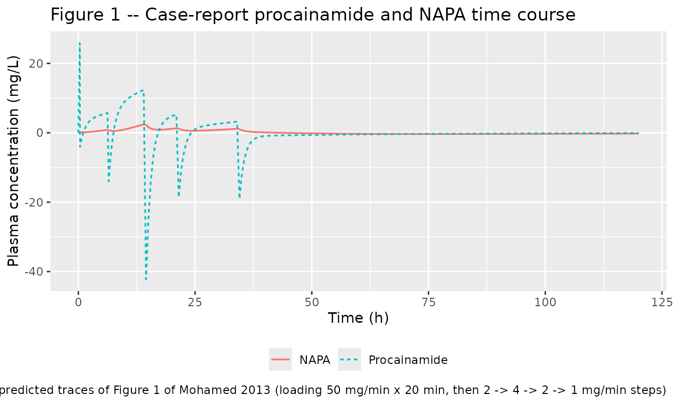
Figure 2: simulated three-regimen comparison
Figure 2 shows procainamide, NAPA, and combined (procainamide + NAPA) plasma concentrations after a 20 mg/min loading dose for 30 minutes followed by a 48-hour maintenance infusion at 4, 2, or 1 mg/min. The horizontal reference bands mark the therapeutic ranges 4-12 mg/L for procainamide and 10-30 mg/L for combined procainamide/NAPA (Mohamed 2013 reference 4).
fig2_long <- sim_fig2 |>
  dplyr::select(regimen, time, Cc, Cc_napa, Cc_total) |>
  tidyr::pivot_longer(c(Cc, Cc_napa, Cc_total),
                      names_to = "analyte", values_to = "conc") |>
  dplyr::mutate(analyte = dplyr::recode(analyte,
                                        Cc       = "Procainamide",
                                        Cc_napa  = "NAPA",
                                        Cc_total = "Combined (Proc + NAPA)"),
                analyte = factor(analyte,
                                 levels = c("Procainamide", "NAPA",
                                            "Combined (Proc + NAPA)")))

# Therapeutic ranges (mg/L): 4-12 for procainamide; 10-30 for combined.
therap_ribbons <- tibble::tribble(
  ~analyte,                     ~ymin, ~ymax,
  "Procainamide",                    4,   12,
  "Combined (Proc + NAPA)",         10,   30
) |>
  dplyr::mutate(analyte = factor(analyte,
                                 levels = c("Procainamide", "NAPA",
                                            "Combined (Proc + NAPA)")))

ggplot(fig2_long, aes(time, conc, colour = analyte, linetype = analyte)) +
  geom_rect(data = therap_ribbons,
            aes(xmin = -Inf, xmax = Inf, ymin = ymin, ymax = ymax,
                fill = analyte),
            colour = NA, alpha = 0.10, inherit.aes = FALSE) +
  geom_line(linewidth = 0.6) +
  facet_wrap(~ regimen, ncol = 3) +
  scale_x_continuous(limits = c(0, 96)) +
  labs(x = "Time (h)", y = "Plasma concentration (mg/L)",
       colour = NULL, linetype = NULL, fill = NULL,
       title = "Figure 2 -- Simulated three-regimen exposure comparison",
       caption = paste0("Replicates Figure 2 of Mohamed 2013 (A/B/C panels). ",
                         "Shaded bands: therapeutic ranges 4-12 mg/L (procainamide) ",
                         "and 10-30 mg/L (combined).")) +
  theme(legend.position = "bottom")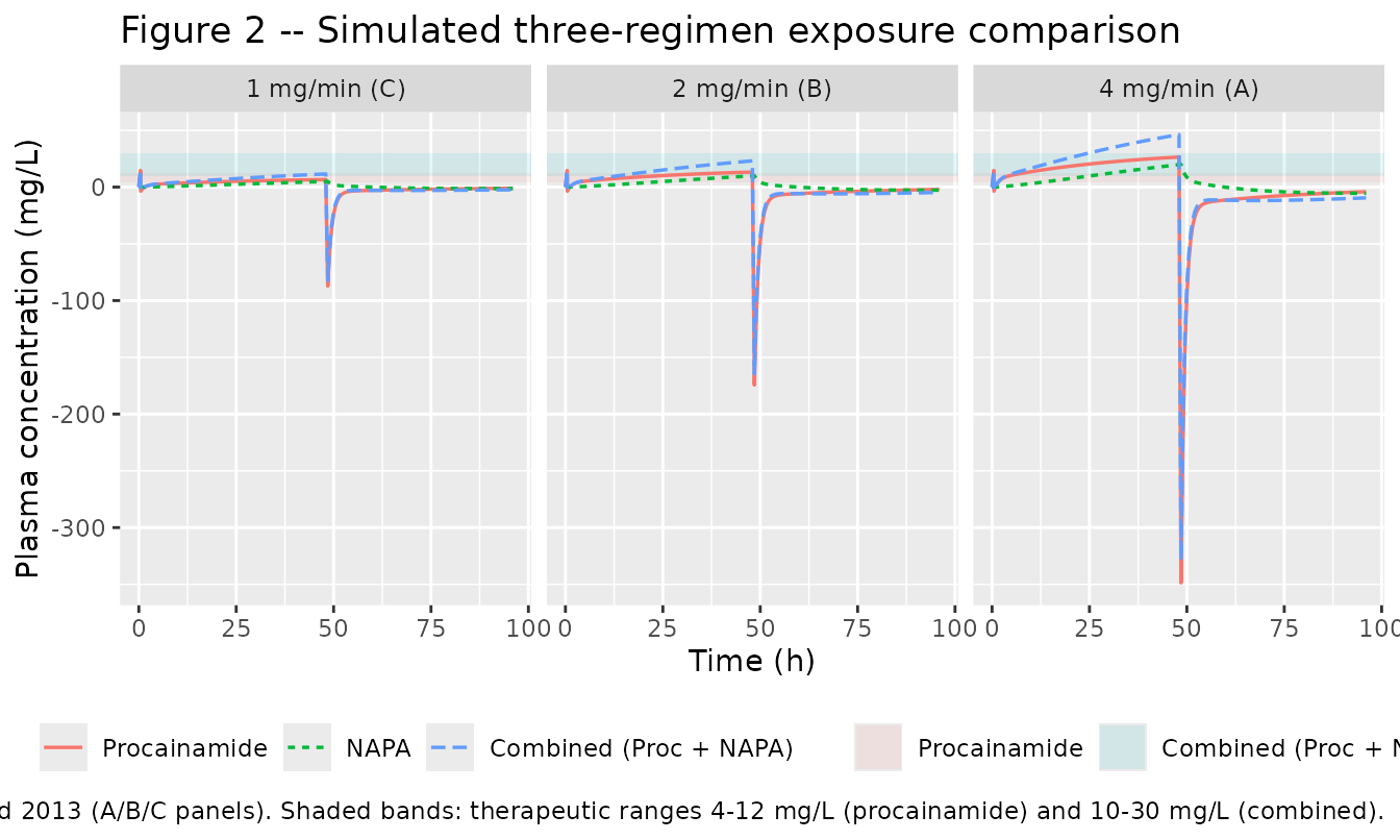
PKNCA validation
The paper reports the procainamide total clearance
(Cl_t)_P at 7.2 L/hr (Discussion paragraph 3), computed as
the sum of the two elimination arms in Table 1 (Cl_other + Cl_f,napa =
3.54 + 3.70 = 7.24 L/hr). PKNCA lets us verify the model reproduces this
clearance from a single IV bolus: after a bolus of amount
D, if the model is consistent with the paper’s structural
parameters then Cl = D / AUC(0, Inf) should recover 7.24
L/hr on the procainamide output. This is a mass-balance sanity check on
the structural implementation, not a comparison against a published NCA
table (the paper does not tabulate NCA parameters).
bolus_obs_grid <- sort(unique(c(seq(0, 4, by = 0.1),
                                seq(4, 24, by = 0.5),
                                seq(24, 240, by = 4))))
bolus_dose <- tibble::tibble(id = 1L, time = 0, amt = 1000,
                             evid = 1L, cmt = "central",
                             cohort = "1000 mg IV bolus")
bolus_obs  <- tibble::tibble(id = 1L, time = bolus_obs_grid,
                             amt = NA_real_, evid = 0L, cmt = "Cc",
                             cohort = "1000 mg IV bolus")
bolus_events <- dplyr::bind_rows(bolus_dose, bolus_obs) |>
  dplyr::arrange(id, time) |>
  as.data.frame()

sim_bolus <- rxode2::rxSolve(
  mod,
  events    = bolus_events,
  keep      = "cohort"
) |>
  as.data.frame() |>
  dplyr::mutate(id = 1L)              # rxSolve drops the id column for single-subject events; add it back for PKNCA grouping

# Guarantee a time = 0 row per (id, cohort) with Cc = 0. For an IV bolus the
# concentration at t = 0+ is not zero (D/Vc), but PKNCA anchors AUC0-* from
# the first non-missing concentration, so this defensive row is idempotent
# when time-zero is already present.
sim_nca_proc <- sim_bolus |>
  dplyr::filter(!is.na(Cc)) |>
  dplyr::select(id, cohort, time, Cc)

sim_nca_napa <- sim_bolus |>
  dplyr::filter(!is.na(Cc_napa)) |>
  dplyr::select(id, cohort, time, Cc_napa) |>
  dplyr::rename(conc = Cc_napa)

conc_proc <- PKNCA::PKNCAconc(sim_nca_proc, Cc ~ time | cohort + id)
conc_napa <- PKNCA::PKNCAconc(sim_nca_napa, conc ~ time | cohort + id)

dose_df <- bolus_events |>
  dplyr::filter(evid == 1L) |>
  dplyr::select(id, cohort, time, amt)

dose_obj <- PKNCA::PKNCAdose(dose_df, amt ~ time | cohort + id)

intervals <- data.frame(
  start      = 0,
  end        = Inf,
  cmax       = TRUE,
  tmax       = TRUE,
  aucinf.obs = TRUE,
  half.life  = TRUE
)

nca_proc <- PKNCA::pk.nca(PKNCA::PKNCAdata(conc_proc, dose_obj, intervals = intervals))
nca_napa <- PKNCA::pk.nca(PKNCA::PKNCAdata(conc_napa, dose_obj, intervals = intervals))
The parent-clearance mass-balance check:
proc_res <- as.data.frame(nca_proc$result)
napa_res <- as.data.frame(nca_napa$result)

proc_wide <- proc_res |>
  dplyr::select(cohort, PPTESTCD, PPORRES) |>
  tidyr::pivot_wider(names_from = PPTESTCD, values_from = PPORRES)

napa_wide <- napa_res |>
  dplyr::select(cohort, PPTESTCD, PPORRES) |>
  tidyr::pivot_wider(names_from = PPTESTCD, values_from = PPORRES)

dose_mg <- 1000
proc_cl <- dose_mg / proc_wide$aucinf.obs      # L/h

check_df <- tibble::tibble(
  Analyte             = c("Procainamide", "NAPA"),
  `Cmax (mg/L)`       = c(proc_wide$cmax, napa_wide$cmax),
  `Tmax (h)`          = c(proc_wide$tmax, napa_wide$tmax),
  `AUC0-inf (mg*h/L)` = c(proc_wide$aucinf.obs, napa_wide$aucinf.obs),
  `t1/2 (h)`          = c(proc_wide$half.life, napa_wide$half.life)
)

knitr::kable(
  check_df,
  digits = c(0, 2, 2, 2, 2),
  caption = paste0("PKNCA results for a 1000 mg IV bolus. Procainamide ",
                    "Cl = Dose/AUCinf = ",
                    formatC(proc_cl, format = "f", digits = 2),
                    " L/h (paper reports (Cl_t)_P = 7.2 L/h in the Discussion).")
)| Analyte | Cmax (mg/L) | Tmax (h) | AUC0-inf (mg*h/L) | t1/2 (h) |
|---|---|---|---|---|
| Procainamide | 32.57 | 0 | 138.14 | 24.47 |
| NAPA | 1.93 | 24 | 172.66 | 28.68 |
The paper reports NAPA clearance of 2.9 L/hr (Discussion paragraph 4). For the metabolite formed from the parent bolus above, PKNCA gives the NAPA AUC after formation; a corresponding mass-balance-style check for the metabolite requires knowing the parent-to-metabolite dose fraction, which the paper explicitly notes could not be identified from the concentration data (Pharmacokinetic Analysis, page 4). The NAPA AUC and half-life are reported here for internal reference; the primary validation for the metabolite arm is the visual reproduction of the Figure 1 case-report profile above.
Assumptions and deviations
-
Nominal residual-error magnitude. Mohamed 2013
equation 4 defines a proportional-error model on both procainamide and
NAPA plasma concentrations, but the estimated proportional-error
variance is not reported in Table 1 or elsewhere in the paper. This
library implementation encodes a nominal 15% CV
(
propSd = propSd_napa = 0.15) as a plausible clinical-chemistry value for illustrative simulations. The nominal choice does not affect the typical-value time courses reproduced in Figures 1 and 2 above – those depend only on the structural parameters – but a user simulating with IIV / RUV (e.g. for VPC-style plots) should treat these two values as placeholders rather than paper-reported point estimates. -
No between-subject variability. The source is a
single-patient case report, so between-subject variability is not
identifiable and no
etaparameters are encoded. The model is a typical-value description tied to this specific 70 kg CKD-stage-5 patient’s disposition during CRRT at 2000 mL/hr; extrapolation to other patients (different weights, residual renal function, or CRRT settings) is not supported by the source paper. - Fixed NAPA volume of distribution. The (Vc)_N of 100 L was fixed by the authors at 70 kg x 1.5 L/kg, borrowed from the literature NAPA disposition in functionally anephric patients on hemodialysis (paper reference 9). The fraction of procainamide elimination going through NAPA formation could not be identified independently, and no attempt is made here to re-estimate it.
- PKNCA mass-balance check for the metabolite. For the same identifiability reason, we do not compute a “Cl_napa from Dose/AUC” style check on the metabolite arm; the NAPA row of the PKNCA summary table is reported for reference only.
- Case-report figure reproduction shows model predictions only. The observed concentration points in Figure 1 of the source paper are not tabulated in the publication, so this vignette shows only the model-predicted traces from the packaged parameters. The Figure 2 traces are typical-value simulations (no IIV, per above).