SHetA2 interspecies scaling (Sharma 2018)
Source:vignettes/articles/Sharma_2018_SHetA2.Rmd
Sharma_2018_SHetA2.RmdModel and source
- Citation: Sharma A, Benbrook DM, Woo S. Pharmacokinetics and interspecies scaling of a novel, orally-bioavailable anti-cancer drug, SHetA2. PLoS ONE 2018;13(4):e0194046.
- Article (open access): doi:10.1371/journal.pone.0194046
The paper develops compartmental PK models for SHetA2 (a flexible
heteroarotinoid anti-cancer / chemoprevention drug) in mouse, rat, and
dog, then applies simple and maximum-life-span-potential (MLP)
allometric scaling to project a typical 70-kg human disposition for
first-in-human dose selection. Four modellib() entries
cover the four scenarios:
-
Sharma_2018_SHetA2_mouse– mouse 2-cmt + first-order absorption. -
Sharma_2018_SHetA2_rat– rat 2-cmt + first-order absorption. -
Sharma_2018_SHetA2_dog– dog 2-cmt + 7-compartment GI transit with two absorption sites (G2 and G7). -
Sharma_2018_SHetA2_human– 70-kg human IV disposition (no parametric oral absorption – the source paper simulated the oral profile externally with the GastroPlus 9.5 ACAT model, which is not reproducible inside nlmixr2lib).
Population and study design
The preclinical PK data were re-analysed from three published preclinical studies (Sharma 2018 Table 1):
- Mouse: CD2F1 female mice, 20.0-27.8 g (n=3 per arm). IV 20 mg/kg in PEG400:Ethanol:Saline; PO 20 and 60 mg/kg in sesame oil by gavage. Cardiac-puncture blood sampling at 16 IV time points and 13 PO time points.
- Rat: Crl:CD Sprague-Dawley rats, 260-347 g (n=3 per arm). IV 5 mg/kg single dose; PO 100, 500, or 2000 mg/kg/day in 1% methylcellulose / 0.2% Tween 80 for 28 days, with PK sampled on the IV day and on week 4 or 5 of the oral arm. Retro-orbital sampling at 8 IV time points and 8 PO time points. Rat PK data were digitized using GetData Graph Digitizer v2.26.
- Beagle dog (NCI N01-CN-43306 toxicology report, work assignment 21): 6.4-11.2 kg (males 9.0-11.2 kg; females 6.9-8.4 kg in the oral arms; IV arm 6.4-7.0 kg). IV 5 mg/kg (n=2, mean only); PO 100, 400, or 1500 mg/kg in 30% aqueous Solutol HS 15 by gavage (n=4 per dose). Jugular sampling at 9 IV time points and 8 PO time points.
All compartmental fits used Phoenix WinNonlin v6.4 with the
Gauss-Newton (Levenberg-Hartley) minimization algorithm and 1/y^2
weighting. Per-species IV and PO data were fit simultaneously by
naive-pooled least squares; the authors did not report
inter-individual variability and the residual error magnitude is not
reported. Population metadata is available programmatically via, for
example,
readModelDb("Sharma_2018_SHetA2_mouse")$population.
Source trace
Per-parameter origin is recorded as in-file comments next to each
ini() entry in
inst/modeldb/specificDrugs/Sharma_2018_SHetA2_{mouse,rat,dog,human}.R.
The table below collects them in one place for review. The reported CV%
values are precisions of the parameter estimates (RSE-like SEs from the
Gauss-Newton fit), NOT inter-individual variability.
| Species | Parameter | Value (CV%) | Source location |
|---|---|---|---|
| Mouse | CL | 0.0421 L/h (8%) | Sharma 2018 Table 3 |
| Mouse | V1 | 0.121 L (16%) | Sharma 2018 Table 3 |
| Mouse | CLD | 0.0323 L/h (20%) | Sharma 2018 Table 3 |
| Mouse | V2 | 0.282 L (14%) | Sharma 2018 Table 3 |
| Mouse | kA | 0.539 1/h (19%) | Sharma 2018 Table 3 |
| Mouse | F (20 mg/kg) | 17.7% (12%) | Sharma 2018 Table 3 |
| Mouse | F (60 mg/kg) | 19.5% (12%) | Sharma 2018 Table 3 |
| Rat | CL | 0.916 L/h (10%) | Sharma 2018 Table 3 |
| Rat | V1 | 0.969 L (18%) | Sharma 2018 Table 3 |
| Rat | CLD | 0.286 L/h (70%) | Sharma 2018 Table 3 |
| Rat | V2 | 0.531 L (48%) | Sharma 2018 Table 3 |
| Rat | kA | 0.0755 1/h (17%) | Sharma 2018 Table 3 |
| Rat | F (100 mg/kg) | 1.03% (14%) | Sharma 2018 Table 3 |
| Rat | F (500 mg/kg) | 1.57% (19%) | Sharma 2018 Table 3 |
| Rat | F (2000 mg/kg) | 0.560% (16%) | Sharma 2018 Table 3 |
| Dog | CL | 6.39 L/h (10%) | Sharma 2018 Table 3 |
| Dog | V1 | 8.53 L (18%) | Sharma 2018 Table 3 |
| Dog | CLD | 3.24 L/h (29%) | Sharma 2018 Table 3 |
| Dog | V2 | 22.5 L (26%) | Sharma 2018 Table 3 |
| Dog | F / kA / kA2 / kAT (100 mg/kg) | 11.2% / 1.12 / 0.929 / 0.532 | Sharma 2018 Table 3 |
| Dog | F / kA / kA2 / kAT (400 mg/kg) | 3.45% / 1.12 / 0.105 / 1.11 | Sharma 2018 Table 3 |
| Dog | F / kA / kA2 / kAT (1500 mg/kg) | 1.11% / 0.411 / 0.0898 / 1.25 | Sharma 2018 Table 3 |
| Human (70 kg) | CL (MLP) | 17.3 L/h | Sharma 2018 Results, Allometric scaling |
| Human (70 kg) | V1 | 36.2 L | Sharma 2018 Results, Prediction of human PK |
| Human (70 kg) | V2 | 68.5 L | Sharma 2018 Results, Prediction of human PK |
| Human (70 kg) | CLD | 15.2 L/h | Sharma 2018 Results, Prediction of human PK |
| Mouse / Rat disposition + 1st-order absorption ODE | n/a | Sharma 2018 Eqs. 1-3 + Fig. 2A | |
| Dog 7-compartment GI transit + dual absorption ODE | n/a | Sharma 2018 Eqs. 4-9 + Fig. 2B | |
| Simple allometry P = a * BW^b across mouse/rat/dog | n/a | Sharma 2018 Allometric scaling + Fig. 5 |
Helpers
A single helper builds an IV-or-oral event table for any species, with one subject per dose. All four species share the same time / dose / concentration units (h, mg, ng/mL), so the helper is species-agnostic.
make_cohort <- function(model_name, dose_mg_kg, body_kg, route, tmax_h = 72,
                        dt_h = 0.05, id_offset = 0L) {
  amt_mg <- dose_mg_kg * body_kg
  cmt_in <- if (route == "IV") "central" else "depot"
  ev <- rxode2::et(amt = amt_mg, cmt = cmt_in) |>
    rxode2::et(seq(0, tmax_h, by = dt_h))
  as.data.frame(ev) |>
    dplyr::mutate(
      id        = id_offset + 1L,
      treatment = sprintf("%s %g mg/kg", route, dose_mg_kg),
      species   = sub("^Sharma_2018_SHetA2_", "", model_name)
    )
}
A second helper runs a typical-value (no residual-error)
rxSolve and tags the rows for cross-species comparison:
run_typical <- function(model_name, dose_mg_kg, body_kg, route, tmax_h = 72,
                        dt_h = 0.05, id_offset = 0L) {
  m  <- nlmixr2lib::readModelDb(model_name) |> rxode2::zeroRe()
  ev <- make_cohort(model_name, dose_mg_kg, body_kg, route,
                    tmax_h = tmax_h, dt_h = dt_h, id_offset = id_offset)
  sim <- rxode2::rxSolve(m, events = ev,
                         keep = c("treatment", "species")) |>
    as.data.frame()
  # rxSolve drops the id column for single-subject runs; restore it from the
  # event table so downstream PKNCA grouping has a valid subject key.
  sim$id         <- id_offset + 1L
  sim$dose_mg_kg <- dose_mg_kg
  sim$route      <- route
  sim
}
Mouse PK – Figure 3A
CD2F1 mice received 20 mg/kg IV and 20 or 60 mg/kg PO; the paper’s Figure 3A shows the three observed concentration-time profiles overlaid with the compartmental fit. The simulation below assumes a typical 24-g female mouse.
mouse_iv20 <- run_typical("Sharma_2018_SHetA2_mouse", 20, 0.024, "IV", id_offset = 0L)
#> Warning: No omega parameters in the model
mouse_po20 <- run_typical("Sharma_2018_SHetA2_mouse", 20, 0.024, "PO", id_offset = 1L)
#> Warning: No omega parameters in the model
mouse_po60 <- run_typical("Sharma_2018_SHetA2_mouse", 60, 0.024, "PO", id_offset = 2L)
#> Warning: No omega parameters in the model
mouse_sim  <- dplyr::bind_rows(mouse_iv20, mouse_po20, mouse_po60)
ggplot(mouse_sim, aes(time, Cc, colour = treatment)) +
  geom_line() +
  scale_y_log10() +
  labs(x = "Time (h)", y = "SHetA2 plasma concentration (ng/mL)",
       title = "Figure 3A -- SHetA2 PK in CD2F1 mouse",
       caption = "Replicates Figure 3A of Sharma 2018.",
       colour = NULL)
#> Warning in scale_y_log10(): log-10 transformation introduced infinite values.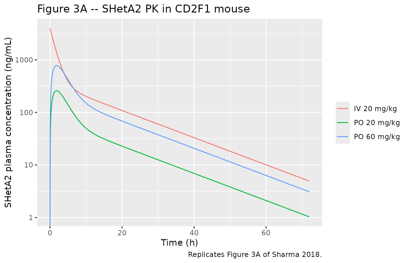
Rat PK – Figure 3B
Crl:CD (SD) rats received 5 mg/kg IV and 100, 500, or 2000 mg/kg PO. The single fitted kA (0.0755 1/h) is dominated by the higher-dose flip-flop kinetics; the lower-dose profile (100 mg/kg) is a coarser fit by design.
rat_iv5    <- run_typical("Sharma_2018_SHetA2_rat",   5,   0.30, "IV", id_offset = 10L, tmax_h = 48)
#> Warning: No omega parameters in the model
rat_po100  <- run_typical("Sharma_2018_SHetA2_rat",   100, 0.30, "PO", id_offset = 11L, tmax_h = 48)
#> Warning: No omega parameters in the model
rat_po500  <- run_typical("Sharma_2018_SHetA2_rat",   500, 0.30, "PO", id_offset = 12L, tmax_h = 48)
#> Warning: No omega parameters in the model
rat_po2000 <- run_typical("Sharma_2018_SHetA2_rat",   2000, 0.30, "PO", id_offset = 13L, tmax_h = 48)
#> Warning: No omega parameters in the model
rat_sim    <- dplyr::bind_rows(rat_iv5, rat_po100, rat_po500, rat_po2000)
ggplot(rat_sim, aes(time, Cc, colour = treatment)) +
  geom_line() +
  scale_y_log10() +
  labs(x = "Time (h)", y = "SHetA2 plasma concentration (ng/mL)",
       title = "Figure 3B -- SHetA2 PK in Crl:CD (SD) rat",
       caption = "Replicates Figure 3B of Sharma 2018.",
       colour = NULL)
#> Warning in scale_y_log10(): log-10 transformation introduced infinite values.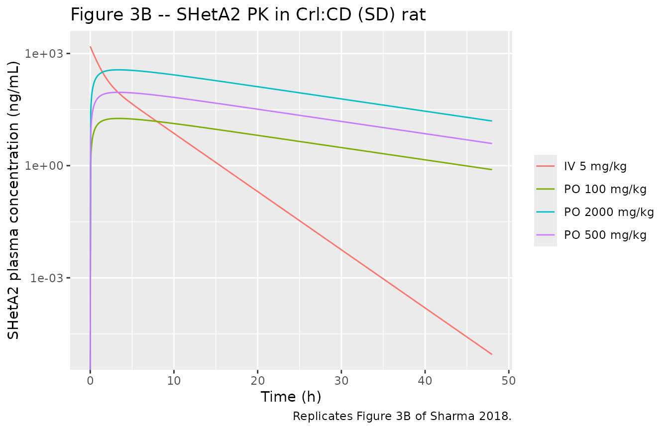
Dog PK – Figure 3C (100 mg/kg subset)
The dog model uses the 100 mg/kg parameter set (F=11.2%, kA=1.12,
kA2=0.929, kAT=0.532). The single early peak observed at 100 mg/kg is
captured by the G2 absorption (kA); at higher doses (400 and 1500 mg/kg)
the model also needs the late G7 absorption (kA2) and a faster transit
(kAT) to capture the double-peak phenomenon, but those parameter sets
are not encoded in this .R file – see Assumptions and
deviations.
dog_iv5    <- run_typical("Sharma_2018_SHetA2_dog", 5,   7, "IV", id_offset = 20L, tmax_h = 48)
#> Warning: No omega parameters in the model
dog_po100  <- run_typical("Sharma_2018_SHetA2_dog", 100, 7, "PO", id_offset = 21L, tmax_h = 48)
#> Warning: No omega parameters in the model
dog_sim    <- dplyr::bind_rows(dog_iv5, dog_po100)
ggplot(dog_sim, aes(time, Cc, colour = treatment)) +
  geom_line() +
  scale_y_log10() +
  labs(x = "Time (h)", y = "SHetA2 plasma concentration (ng/mL)",
       title = "Figure 3C -- SHetA2 PK in beagle dog (IV + 100 mg/kg PO)",
       caption = "Subset of Figure 3C of Sharma 2018 (100 mg/kg arm only).",
       colour = NULL)
#> Warning in scale_y_log10(): log-10 transformation introduced infinite values.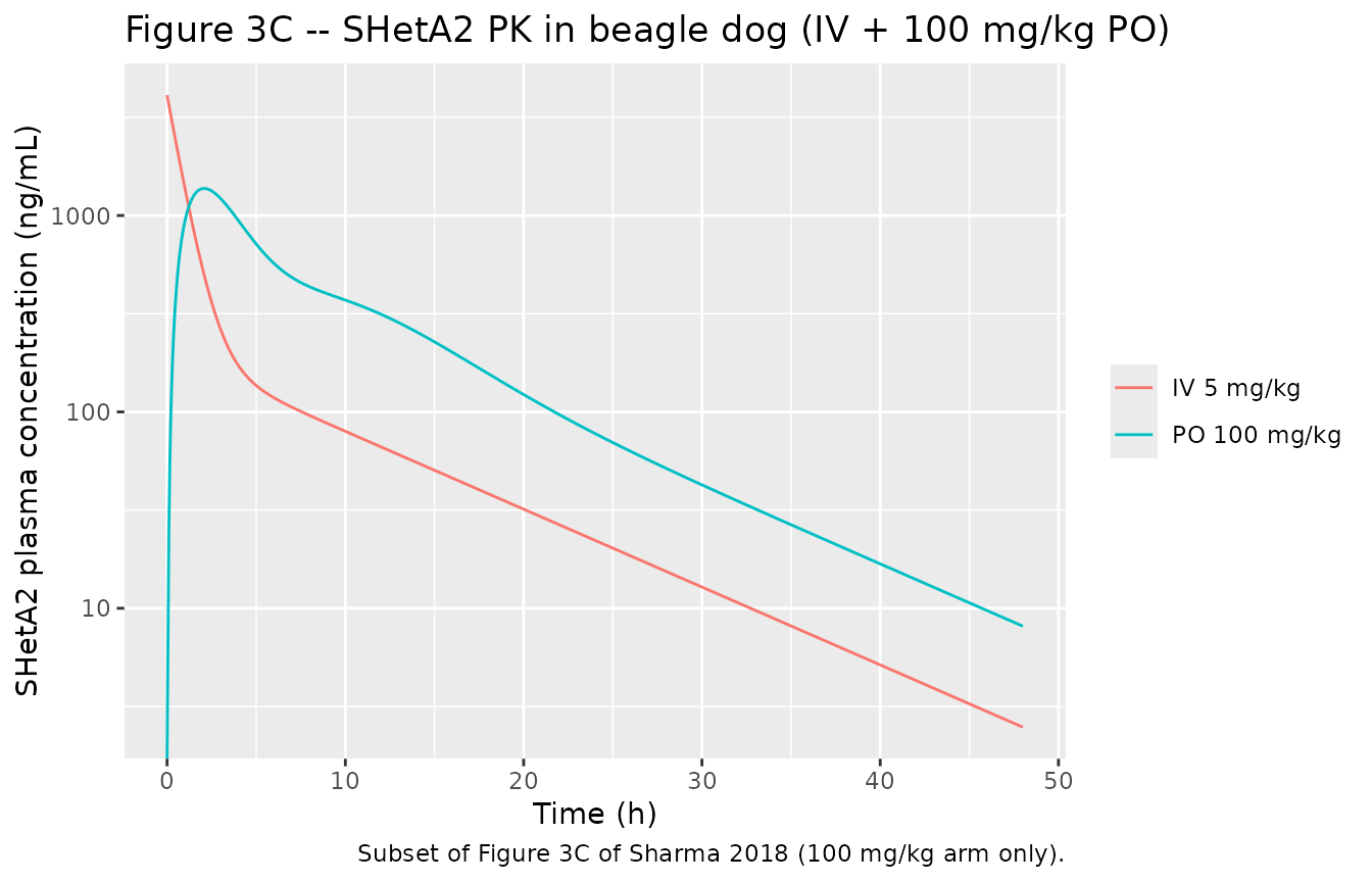
PKNCA validation against Sharma 2018 Table 2
Per pknca-recipes.md, the formula carries a treatment
grouping so the comparison can be made per-dose against the paper’s NCA
table.
all_sim <- dplyr::bind_rows(mouse_sim, rat_sim, dog_sim) |>
  dplyr::mutate(group = paste(species, treatment, sep = " | "))

# Build the dose data frame from the events
all_events <- dplyr::bind_rows(
  make_cohort("Sharma_2018_SHetA2_mouse", 20, 0.024, "IV", id_offset = 0L),
  make_cohort("Sharma_2018_SHetA2_mouse", 20, 0.024, "PO", id_offset = 1L),
  make_cohort("Sharma_2018_SHetA2_mouse", 60, 0.024, "PO", id_offset = 2L),
  make_cohort("Sharma_2018_SHetA2_rat",   5,   0.30, "IV", id_offset = 10L),
  make_cohort("Sharma_2018_SHetA2_rat",   100, 0.30, "PO", id_offset = 11L),
  make_cohort("Sharma_2018_SHetA2_rat",   500, 0.30, "PO", id_offset = 12L),
  make_cohort("Sharma_2018_SHetA2_rat",   2000, 0.30, "PO", id_offset = 13L),
  make_cohort("Sharma_2018_SHetA2_dog",   5,   7,    "IV", id_offset = 20L),
  make_cohort("Sharma_2018_SHetA2_dog",   100, 7,    "PO", id_offset = 21L)
) |>
  dplyr::mutate(group = paste(species, treatment, sep = " | "))

sim_nca <- all_sim |>
  dplyr::filter(!is.na(Cc)) |>
  dplyr::select(id, time, Cc, group)

# Defensive time-zero row (extravascular Cc=0 is the right pre-dose value;
# for the IV arm the row already exists from rxSolve).
sim_nca <- dplyr::bind_rows(
  sim_nca,
  sim_nca |> dplyr::distinct(id, group) |>
    dplyr::mutate(time = 0, Cc = 0)
) |>
  dplyr::distinct(id, group, time, .keep_all = TRUE) |>
  dplyr::arrange(id, group, time)

dose_df <- all_events |>
  dplyr::filter(evid == 1) |>
  dplyr::select(id, time, amt, group)

conc_obj <- PKNCA::PKNCAconc(sim_nca, Cc ~ time | group + id,
                             concu = "ng/mL", timeu = "h")
dose_obj <- PKNCA::PKNCAdose(dose_df, amt ~ time | group + id,
                             doseu = "mg")

intervals <- data.frame(
  start       = 0,
  end         = Inf,
  cmax        = TRUE,
  tmax        = TRUE,
  aucinf.obs  = TRUE,
  half.life   = TRUE
)

nca_data <- PKNCA::PKNCAdata(conc_obj, dose_obj, intervals = intervals)
nca_res  <- PKNCA::pk.nca(nca_data)
Comparison against Sharma 2018 Table 2
published <- tibble::tribble(
  ~group,                ~cmax, ~tmax, ~aucinf.obs, ~half.life,
  "mouse | IV 20 mg/kg", 4370,  0.1,   10942,       11.5,
  "mouse | PO 20 mg/kg", 316,   2.0,   1801,        10.8,
  "mouse | PO 60 mg/kg", 944,   3.0,   6875,        7.02,
  "rat | IV 5 mg/kg",    1642,  0.1,   1583,        1.16,
  "rat | PO 100 mg/kg",  55,    2.0,   542,         10.4,
  "rat | PO 500 mg/kg",  195,   6.0,   1413,        NA_real_,
  "rat | PO 2000 mg/kg", 231,   6.0,   3586,        7.49,
  "dog | IV 5 mg/kg",    4034,  0.1,   4885,        6.93,
  "dog | PO 100 mg/kg",  2004,  3.0,   16813,       6.77
)

cmp <- nlmixr2lib::ncaComparisonTable(
  simulated     = nca_res,
  reference     = published,
  by            = "group",
  units         = c(cmax = "ng/mL", aucinf.obs = "ng*h/mL",
                    tmax = "h", half.life = "h"),
  tolerance_pct = 30
)

knitr::kable(
  cmp,
  caption = paste(
    "Simulated typical-value NCA vs. Sharma 2018 Table 2 published NCA.",
    "* differs from reference by >30%. Note: PO comparisons at higher rat",
    "and dog doses are expected to differ because (a) the rat compartmental",
    "fit used a single kA = 0.0755 1/h driven by the higher-dose flip-flop",
    "kinetics (Cmax/Tmax at 100 mg/kg is therefore dose-mismatched), and",
    "(b) the dog model is encoded at the 100 mg/kg parameter set only."
  )
)| NCA parameter | group | Reference | Simulated | % diff |
|---|---|---|---|---|
| Cmax (ng/mL) | mouse | IV 20 mg/kg | 4370 | 3970 | -9.2% |
| Cmax (ng/mL) | mouse | PO 20 mg/kg | 316 | 259 | -18.1% |
| Cmax (ng/mL) | mouse | PO 60 mg/kg | 944 | 776 | -17.8% |
| Cmax (ng/mL) | rat | IV 5 mg/kg | 1640 | 1550 | -5.7% |
| Cmax (ng/mL) | rat | PO 100 mg/kg | 55 | 18.3 | -66.8%* |
| Cmax (ng/mL) | rat | PO 500 mg/kg | 195 | 91.4 | -53.1%* |
| Cmax (ng/mL) | rat | PO 2000 mg/kg | 231 | 366 | +58.3%* |
| Cmax (ng/mL) | dog | IV 5 mg/kg | 4030 | 4100 | +1.7% |
| Cmax (ng/mL) | dog | PO 100 mg/kg | 2000 | 1370 | -31.5%* |
| Tmax (h) | mouse | IV 20 mg/kg | 0.1 | 0 | -100.0%* |
| Tmax (h) | mouse | PO 20 mg/kg | 2 | 1.8 | -10.0% |
| Tmax (h) | mouse | PO 60 mg/kg | 3 | 1.8 | -40.0%* |
| Tmax (h) | rat | IV 5 mg/kg | 0.1 | 0 | -100.0%* |
| Tmax (h) | rat | PO 100 mg/kg | 2 | 3.4 | +70.0%* |
| Tmax (h) | rat | PO 500 mg/kg | 6 | 3.4 | -43.3%* |
| Tmax (h) | rat | PO 2000 mg/kg | 6 | 3.4 | -43.3%* |
| Tmax (h) | dog | IV 5 mg/kg | 0.1 | 0 | -100.0%* |
| Tmax (h) | dog | PO 100 mg/kg | 3 | 2.1 | -30.0% |
| AUC0-∞ (obs) (ng*h/mL) | mouse | IV 20 mg/kg | 10900 | 11400 | +4.2% |
| AUC0-∞ (obs) (ng*h/mL) | mouse | PO 20 mg/kg | 1800 | 2120 | +17.7% |
| AUC0-∞ (obs) (ng*h/mL) | mouse | PO 60 mg/kg | 6880 | 6360 | -7.5% |
| AUC0-∞ (obs) (ng*h/mL) | rat | IV 5 mg/kg | 1580 | 1640 | +3.5% |
| AUC0-∞ (obs) (ng*h/mL) | rat | PO 100 mg/kg | 542 | 337 | -37.7%* |
| AUC0-∞ (obs) (ng*h/mL) | rat | PO 500 mg/kg | 1410 | 1690 | +19.4% |
| AUC0-∞ (obs) (ng*h/mL) | rat | PO 2000 mg/kg | 3590 | 6750 | +88.2%* |
| AUC0-∞ (obs) (ng*h/mL) | dog | IV 5 mg/kg | 4880 | 5480 | +12.1% |
| AUC0-∞ (obs) (ng*h/mL) | dog | PO 100 mg/kg | 16800 | 10800 | -35.6%* |
| t½ (h) | mouse | IV 20 mg/kg | 11.5 | 11.6 | +0.9% |
| t½ (h) | mouse | PO 20 mg/kg | 10.8 | 11.6 | +7.3% |
| t½ (h) | mouse | PO 60 mg/kg | 7.02 | 11.6 | +65.1%* |
| t½ (h) | rat | IV 5 mg/kg | 1.16 | 1.93 | +66.1%* |
| t½ (h) | rat | PO 100 mg/kg | 10.4 | 9.26 | -11.0% |
| t½ (h) | rat | PO 500 mg/kg | — | 9.26 | — |
| t½ (h) | rat | PO 2000 mg/kg | 7.49 | 9.26 | +23.6% |
| t½ (h) | dog | IV 5 mg/kg | 6.93 | 7.57 | +9.2% |
| t½ (h) | dog | PO 100 mg/kg | 6.77 | 7.49 | +10.6% |
Discrepancies in this table are expected for the lower-dose rat (the compartmental kA is averaged over three doses and is dominated by the higher-dose flip-flop kinetics) and for the dog 100 mg/kg PO Cmax (the paper noted only that the model “captured the observed plasma concentration-time profiles reasonably well” – there is no published exact-NCA-match expectation).
Allometric scaling – Figure 5 (text reproduction)
The paper applies simple allometry P = a * BW^b on a log-log plot across mouse / rat / dog disposition values to scale to a 70-kg human. The fitted exponents and the resulting human-projected values come straight from Results (Allometric scaling and Prediction of human pharmacokinetics):
species_bw <- tibble::tribble(
  ~species,        ~BW_kg, ~CL,     ~V1,    ~CLD,    ~V2,
  "mouse (24 g)",  0.024,  0.0421,  0.121,  0.0323,  0.282,
  "rat (300 g)",   0.300,  0.916,   0.969,  0.286,   0.531,
  "dog (7 kg)",    7.000,  6.390,   8.530,  3.240,   22.500,
  "human (70 kg, simple allom.)", 70, 41.0, 36.2,    15.2,    68.5,
  "human (70 kg, MLP-corrected)", 70, 17.3, 36.2,    15.2,    68.5
)

knitr::kable(
  species_bw,
  caption = paste(
    "Per-species disposition values used as inputs to the allometric",
    "regressions (Sharma 2018 Fig. 5 and Allometric scaling section).",
    "The packaged Sharma_2018_SHetA2_human model encodes the MLP-corrected",
    "row (CL = 17.3 L/h) because simple allometry overpredicts human CL",
    "for hepatically-metabolised small molecules."
  )
)| species | BW_kg | CL | V1 | CLD | V2 |
|---|---|---|---|---|---|
| mouse (24 g) | 0.024 | 0.0421 | 0.121 | 0.0323 | 0.282 |
| rat (300 g) | 0.300 | 0.9160 | 0.969 | 0.2860 | 0.531 |
| dog (7 kg) | 7.000 | 6.3900 | 8.530 | 3.2400 | 22.500 |
| human (70 kg, simple allom.) | 70.000 | 41.0000 | 36.200 | 15.2000 | 68.500 |
| human (70 kg, MLP-corrected) | 70.000 | 17.3000 | 36.200 | 15.2000 | 68.500 |
Human PK projection – Figure 6
The packaged Sharma_2018_SHetA2_human model has IV
disposition only. A 10 mg/kg IV bolus in an 85-kg subject (Sharma 2018
Discussion’s escalation target) gives the disposition-only PK profile
below; the paper’s Figure 6 used a GastroPlus 9.5 ACAT-coupled
simulation of the PO route, which is not reproducible here.
human_iv <- run_typical("Sharma_2018_SHetA2_human", 10, 85, "IV",
                        id_offset = 30L, tmax_h = 72, dt_h = 0.1)
#> Warning: No omega parameters in the model
ggplot(human_iv, aes(time, Cc)) +
  geom_line() +
  scale_y_log10() +
  labs(x = "Time (h)", y = "SHetA2 plasma concentration (ng/mL)",
       title = "Allometric human projection -- 10 mg/kg IV in 85-kg subject",
       caption = "Disposition-only equivalent of Sharma 2018 Fig 6 (paper used GastroPlus ACAT for the oral route).")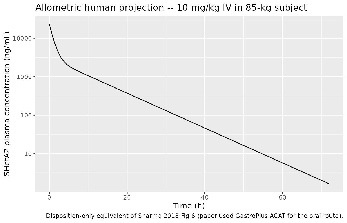
Assumptions and deviations
-
Dose-dependent bioavailability F (mouse, rat, dog).
The paper estimated F separately at each oral dose level: mouse 17.7% /
19.5% at 20 / 60 mg/kg, rat 1.03% / 1.57% / 0.560% at 100 / 500 / 2000
mg/kg, dog 11.2% / 3.45% / 1.11% at 100 / 400 / 1500 mg/kg. The packaged
.Rfiles encode a single “typical” F per species (mouse 18.6%, the Fig. 4 caption summary; rat 1.03%, the 100 mg/kg value as closest to the unsaturated regime; dog 11.2%, the new NOAEL dose) for downstream simulation. Users who need an exact-dose simulation should editlfdepot(and for dog, alsolka,lka2,lktr) to match the desired dose row in Table 3. -
Dog dose-dependent absorption parameters. Beyond F,
the paper estimated kA, kA2, and kAT separately for each oral dose. The
packaged
Sharma_2018_SHetA2_dogmodel encodes only the 100 mg/kg set. The 400 mg/kg set is (F=3.45%, kA=1.12, kA2=0.105, kAT=1.11); the 1500 mg/kg set is (F=1.11%, kA=0.411, kA2=0.0898, kAT=1.25). The CV% on dog kA2 at 100 mg/kg is reported as 281% (Sharma 2018 Table 3), which already signals poor identifiability of the late-absorption arm at this dose. - Rat compartmental fit at 100 mg/kg. The paper used a single kA = 0.0755 1/h across all three rat oral doses, which is dominated by the higher-dose flip-flop kinetics and underestimates the observed early Cmax at 100 mg/kg (paper Table 2: 55 ng/mL at Tmax 2 h vs. fitted ~18 ng/mL at Tmax ~3.4 h). This is a property of the paper’s fit, not a translation defect.
-
No IIV or fitted residual error. The paper used
Phoenix WinNonlin with naive-pooled least squares and 1/y^2 weighting;
neither IIV nor the residual-error magnitude is reported. The packaged
models have no
etaparameters and use a fixed placeholderpropSd = 0.10(10% CV proportional) so that downstreamrxSolve/ PKNCA simulation works. Users who want a deterministic typical-value profile should callrxode2::zeroRe()(therun_typical()helper above does this). -
Human absorption is unmodelled. The paper’s human
oral simulation used GastroPlus 9.5 ACAT (a physiologically-based gut
model not reproducible inside nlmixr2lib). The packaged
Sharma_2018_SHetA2_humanmodel contains the IV disposition only – CL = 17.3 L/h (MLP-corrected allometry), V1 = 36.2 L, V2 = 68.5 L, CLD = 15.2 L/h. Users who want an oral profile should run GastroPlus externally or substitute a paper-anchored proxy kA (e.g. 0.539 1/h, the mouse value used by the GastroPlus-predicted bioavailability of 18.8% in Figure 6). - Body weight is not a model covariate. All species-specific disposition values are reported as absolute (L, L/h) at the typical body weight of the studied animals (mouse 0.024 kg, rat 0.30 kg, dog ~7 kg, human 70 kg). To use the model at a different body weight the user should apply allometric scaling externally; the paper’s fitted exponents come from Fig. 5 (R^2 = 0.91-0.99 across CL / V1 / V2 / CLD).
- Errata. A search of the PLOS ONE landing page and a PubMed search for “Sharma 2018 SHetA2 erratum” on the task-execution date returned no errata or corrections.