Dalbavancin (Baiardi 2025)
Source:vignettes/articles/Baiardi_2025_dalbavancin.Rmd
Baiardi_2025_dalbavancin.RmdModel and source
- Citation: Baiardi G, Cameran Caviglia M, Boni S, Di Paolo A, Marini V, Cangemi G, Cafaro A, Pontali E, Mattioli F. Multidose Dalbavancin Population Pharmacokinetic Analysis for Prolonged Target Attainment in Patients Requiring Long-Term Treatment. Antibiotics. 2025;14(2):190. doi:10.3390/antibiotics14020190.
- Description: Two-compartment population PK model with first-order elimination for intravenous dalbavancin in adult patients receiving multidose (off-label, long-term) regimens for difficult-to-treat Gram-positive infections with creatinine clearance above 30 mL/min. Total body weight is scaled by allometry with exponents fixed a priori at 0.75 on the clearances (CL, Q) and 1 on the volumes (V1, V2); no other covariate improved the fit, including creatinine clearance. Unbound concentration is returned as Ccu using the reported 7 percent free fraction, because the paper’s PK/PD target is 100 percent fT above 4x MIC (total dalbavancin above 14.29 mg/L at the 0.25 mg/L EUCAST/USCAST breakpoint).
- Article: Antibiotics 2025;14(2):190 (open access, CC BY 4.0)
Dalbavancin is a long-acting lipoglycopeptide whose terminal half-life of about two weeks makes it attractive for outpatient treatment of infections that would otherwise need six weeks or more of daily intravenous therapy. Its only approved indication is acute bacterial skin and skin structure infection, so multidose off-label regimens for osteoarticular, prosthetic-joint and endovascular infection have no established schedule. Baiardi 2025 fitted a population PK model to therapeutic-drug-monitoring data from 30 such patients and used it to work out when the next dose is due.
Population
Thirty adults treated at Ente Ospedaliero Ospedali Galliera (Genoa, Italy) between February 2023 and February 2024 contributed 195 total plasma dalbavancin concentrations (Baiardi 2025 Table 1 and Results 2.2). All had a documented or suspected Gram-positive infection that had failed primary antimicrobial therapy; sites included ABSSSI (10), spondylodiscitis (9), septic arthritis (5) and endocarditis (2). Twenty-one were male and nine female. Median age was 72 years (range 26-97), median weight 72 kg (44-179 kg) and median creatinine clearance by Cockcroft-Gault 66.2 mL/min (31.7-283 mL/min) - every patient was above the 30 mL/min threshold below which the label requires dose reduction.
Each patient received at least two 1500 mg intravenous doses (30-minute infusions) 7 to 14 days apart, with the number and timing of later doses left to the treating physician; the median was 3 doses (range 2-10) with a median of 5.5 TDM samples per patient (range 2-20). Sampling was a trough plus an end-of-infusion peak at each administration, supplemented by sparse samples where feasible. Five concentrations with conditional weighted residuals above 3 were excluded during model building.
The same information is available programmatically via the model’s
population metadata
(readModelDb("Baiardi_2025_dalbavancin")()$population).
Source trace
The per-parameter origin is recorded as an in-file comment next to
each ini() entry in
inst/modeldb/specificDrugs/Baiardi_2025_dalbavancin.R. The
table below collects them in one place for review.
| Equation / parameter | Value | Source location |
|---|---|---|
lcl (CL) |
0.0273 L/h | Table 2, “Final model parameters estimate” (RSE 5.1%; bootstrap 0.0272, CI 0.0251-0.0294) |
lvc (V1) |
3.6 L | Table 2 (RSE 3.7%; bootstrap 3.6, CI 3.4-3.8) |
lq (Q) |
0.0225 L/h | Table 2 (RSE 28.4%; bootstrap 0.0223, CI 0.0175-0.02936) |
lvp (V2) |
6.4 L | Table 2 (RSE 11.9%; bootstrap 6.5, CI 5.6-7.5) |
e_wt_cl_q |
0.75 (fixed) | Results 2.2: “fixed exponents of 0.75 on clearances (CL, Q)” |
e_wt_vc_vp |
1 (fixed) | Results 2.2: “and of 1 on volumes of distribution (V1, V2)” |
fu |
0.07 (fixed) | Discussion: “assuming a 7% free fraction of DAL in plasma”; total 14.29 mg/L equals free 1 mg/L |
etalcl |
0.047265 = log(0.22^2 + 1) | Table 2, Random Effects (CV%): omega CL = 22% (shrinkage 8%) |
etalvc |
0.029490 = log(0.173^2 + 1) | Table 2: omega V1 = 17.3% (shrinkage 17%) |
etalq |
0.271919 = log(0.559^2 + 1) | Table 2: omega Q = 55.9% (shrinkage 30%) |
etalvp |
0.086729 = log(0.301^2 + 1) | Table 2: omega V2 = 30.1% (shrinkage 34%) |
propSd |
0.144 | Table 2, Residual Variability: b (proportional) = 0.144 (RSE 10%) |
| Two-compartment first-order elimination, IV | n/a | Results 2.2: “A two-compartmental model with first-order elimination best described the DAL PK” |
| Allometry about a 70 kg standard | n/a | Results 2.2 plus its allometry references (Holford 1996; Anderson & Holford 2008; Holford & Anderson 2017), which define the 70 kg size standard - see Assumptions below |
| PK/PD target 100% fT > 4x MIC, MIC 0.25 mg/L | free 1 mg/L | Results 2.3 and Methods 4.4 (EUCAST/USCAST clinical breakpoint) |
| Reference regimen 1500 mg day 0 + 1500 mg day 7 | n/a | Results 2.3 and Methods 4.4 |
Creatinine clearance, age, height, serum albumin, serum creatinine
and C-reactive protein were all screened and none was retained; they are
recorded in the model file’s covariatesDataExcluded list.
Notably, adding creatinine clearance to clearance changed the objective
function value by only 0.02 units (Results 2.2).
Virtual cohort
Original observed data are not publicly available (Data Availability Statement). Baiardi 2025 simulated 100,000 profiles from a virtual population of 3000 adults in three weight bands (1000 each) spanning 40-200 kg, with covariates harvested from NHANES so that they stayed physiologically coherent. Weight is the only covariate in the model, so the cohort below reproduces the three weight bands with 200 subjects each (the per-arm cap for these vignettes) and draws weight uniformly within each band. The consequences of that simplification are examined in the weight-sensitivity section below.
set.seed(20250213)

n_per_band <- 200L

bands <- tibble::tribble(
  ~band,        ~wt_lo, ~wt_hi, ~dose3_week,
  "40-80 kg",       40,     80,           5,
  "80-120 kg",      80,    120,           4,
  "120-200 kg",    120,    200,           3
)

# `dose3_week` is the week at which Baiardi 2025 places the third 1500 mg dose
# for that band, i.e. the last week at which the two-dose regimen still held
# PTA above 90% (Results 2.3).

hours_per_week <- 168

# Body weights are drawn once per band and reused across every regimen below,
# so the two-dose and three-dose comparisons run on the same virtual subjects.
band_weights <- lapply(seq_len(nrow(bands)), function(i) {
  stats::runif(n_per_band, bands$wt_lo[i], bands$wt_hi[i])
})
names(band_weights) <- bands$band

# Build one band's event table. `id_offset` keeps subject IDs disjoint across
# bands; rxSolve keys subjects on `id`, so colliding IDs would silently merge
# two subjects into one that receives the summed dose.
make_band <- function(band, wt, dose_times, obs_times, id_offset) {
  stopifnot(length(wt) == n_per_band)
  dosing <- tidyr::expand_grid(
    subj = seq_len(n_per_band),
    time = dose_times
  ) |>
    dplyr::mutate(amt = 1500, evid = 1L, dur = 0.5, cmt = "central")
  obs <- tidyr::expand_grid(
    subj = seq_len(n_per_band),
    time = obs_times
  ) |>
    dplyr::mutate(amt = NA_real_, evid = 0L, dur = NA_real_, cmt = "central")
  dplyr::bind_rows(dosing, obs) |>
    dplyr::mutate(
      id   = id_offset + subj,
      WT   = wt[subj],
      band = band
    ) |>
    dplyr::select(id, time, amt, evid, dur, cmt, WT, band) |>
    dplyr::arrange(id, time, dplyr::desc(evid))
}
The observation grid runs to week 11 at 12-hour resolution, which is ample for a drug whose terminal half-life is around two weeks.
obs_grid <- seq(0, 11 * hours_per_week, by = 12)

# Regimen A - the paper's initial regimen: 1500 mg on day 0 and day 7.
events_2dose <- dplyr::bind_rows(
  lapply(seq_len(nrow(bands)), function(i) {
    make_band(
      band       = bands$band[i],
      wt         = band_weights[[i]],
      dose_times = c(0, hours_per_week),
      obs_times  = obs_grid,
      id_offset  = (i - 1L) * n_per_band
    )
  })
)

# Regimen B - regimen A plus a third 1500 mg dose at the band-specific time
# point identified by the paper's PTA analysis.
events_3dose <- dplyr::bind_rows(
  lapply(seq_len(nrow(bands)), function(i) {
    make_band(
      band       = bands$band[i],
      wt         = band_weights[[i]],
      dose_times = c(0, hours_per_week, bands$dose3_week[i] * hours_per_week),
      obs_times  = obs_grid,
      id_offset  = (i - 1L) * n_per_band
    )
  })
)

stopifnot(!anyDuplicated(unique(events_2dose[, c("id", "time", "evid")])))
stopifnot(!anyDuplicated(unique(events_3dose[, c("id", "time", "evid")])))
Simulation
mod <- readModelDb("Baiardi_2025_dalbavancin")

sim_2dose <- rxode2::rxSolve(
  mod, events = events_2dose, keep = c("WT", "band")
) |>
  as.data.frame() |>
  dplyr::filter(!is.na(Cc))
#> ℹ parameter labels from comments will be replaced by 'label()'

sim_3dose <- rxode2::rxSolve(
  mod, events = events_3dose, keep = c("WT", "band")
) |>
  as.data.frame() |>
  dplyr::filter(!is.na(Cc))

band_levels <- bands$band
sim_2dose$band <- factor(sim_2dose$band, levels = band_levels)
sim_3dose$band <- factor(sim_3dose$band, levels = band_levels)

stopifnot(dplyr::n_distinct(sim_2dose$id) == 3L * n_per_band)
stopifnot(dplyr::n_distinct(sim_3dose$id) == 3L * n_per_band)
Cc is total plasma dalbavancin and Ccu the
free concentration (Ccu = Cc * fu). The paper’s PK/PD
target is 100% fT above 4x MIC with the MIC set at the 0.25 mg/L
EUCAST/USCAST clinical breakpoint, i.e. a free concentration at or above
1 mg/L for the whole treatment period.
mic <- 0.25          # mg/L, EUCAST/USCAST clinical breakpoint (Methods 4.4)
target_free <- 4 * mic  # 1 mg/L free dalbavancin

fu_model <- rxode2::rxode(mod)$theta[["fu"]]
#> ℹ parameter labels from comments will be replaced by 'label()'
target_total <- target_free / fu_model
The corresponding total concentration is 14.29 mg/L, reproducing the 14.29 mg/L TDM threshold the paper derives in its Discussion and recommends in its Conclusions.
Replicate published figures
Figure 3 - PTA of the two-dose regimen by weight band
Because concentrations decline monotonically after the last dose, “100% fT above 4x MIC through week k” is equivalent to “free concentration at week k is at or above 1 mg/L”. PTA at week k is therefore the proportion of subjects still above target at that time.
pta_by_week <- function(sim, weeks) {
  sim |>
    dplyr::filter(time %in% (weeks * hours_per_week)) |>
    dplyr::group_by(band, week = time / hours_per_week) |>
    dplyr::summarise(pta = 100 * mean(Ccu >= target_free), .groups = "drop")
}
# Replicates Figure 3 of Baiardi 2025: PTA% of 1500 mg on day 0 and day 7,
# by weight class.
pta_2dose <- pta_by_week(sim_2dose, 1:11)

ggplot(pta_2dose, aes(week, pta, colour = band)) +
  geom_hline(yintercept = 90, linetype = "dashed") +
  geom_line() +
  geom_point() +
  scale_x_continuous(breaks = 1:11) +
  labs(
    x = "Week", y = "PTA (%) of 100% fT > 4x MIC", colour = "Weight band",
    title = "Figure 3 - PTA of 1500 mg on day 0 + 1500 mg on day 7",
    caption = "Replicates Figure 3 of Baiardi 2025. Dashed line: the 90% PTA criterion."
  )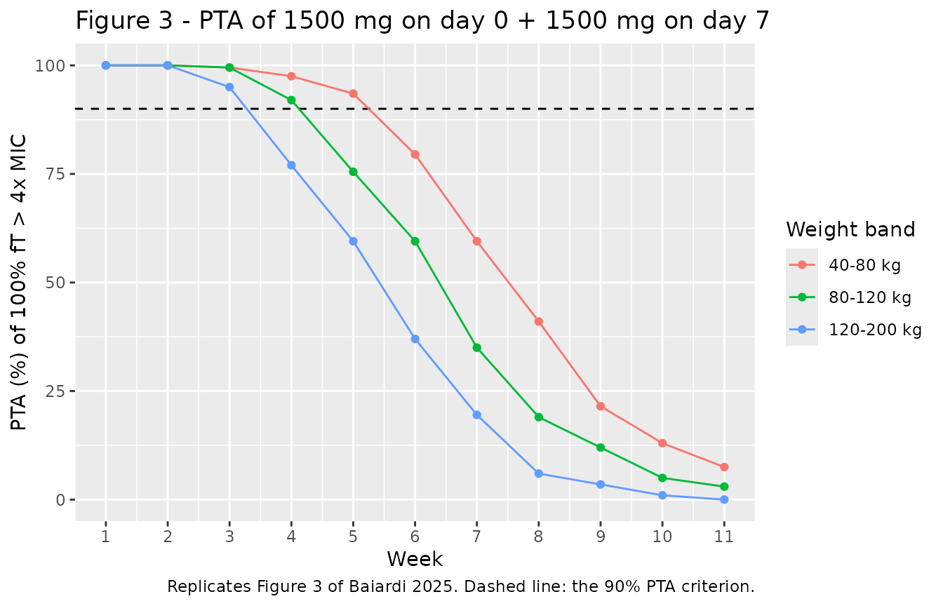
The paper’s claim is that this regimen holds PTA above 90% for 5, 4 and 3 weeks in the 40-80, 80-120 and 120-200 kg bands respectively (Results 2.3). The table below reads the last such week off the simulation and compares it with the paper.
last_week_above <- function(pta_tbl, threshold = 90) {
  pta_tbl |>
    dplyr::filter(pta > threshold) |>
    dplyr::group_by(band) |>
    dplyr::summarise(last_week = max(week), .groups = "drop")
}

cmp_2dose <- last_week_above(pta_2dose) |>
  dplyr::left_join(
    tibble::tibble(band = band_levels, published = c(5, 4, 3)),
    by = "band"
  ) |>
  dplyr::left_join(
    pta_2dose |> dplyr::rename(published_wk = week, pta_at_published = pta),
    by = c("band", "published" = "published_wk")
  ) |>
  dplyr::arrange(match(band, band_levels))

stopifnot(nrow(cmp_2dose) == 3L)

cmp_2dose |>
  dplyr::mutate(pta_at_published = round(pta_at_published, 1)) |>
  dplyr::rename(
    "Weight band"                      = band,
    "Simulated last week with PTA >90%" = last_week,
    "Published (Results 2.3)"           = published,
    "Simulated PTA (%) at that week"    = pta_at_published
  ) |>
  knitr::kable(
    caption = "Figure 3 replication: duration of target attainment for the two-dose regimen."
)| Weight band | Simulated last week with PTA >90% | Published (Results 2.3) | Simulated PTA (%) at that week |
|---|---|---|---|
| 40-80 kg | 5 | 5 | 93.5 |
| 80-120 kg | 4 | 4 | 92.0 |
| 120-200 kg | 3 | 3 | 95.0 |
# The reproduction is exact in all three bands.
stopifnot(identical(as.numeric(cmp_2dose$last_week), as.numeric(cmp_2dose$published)))
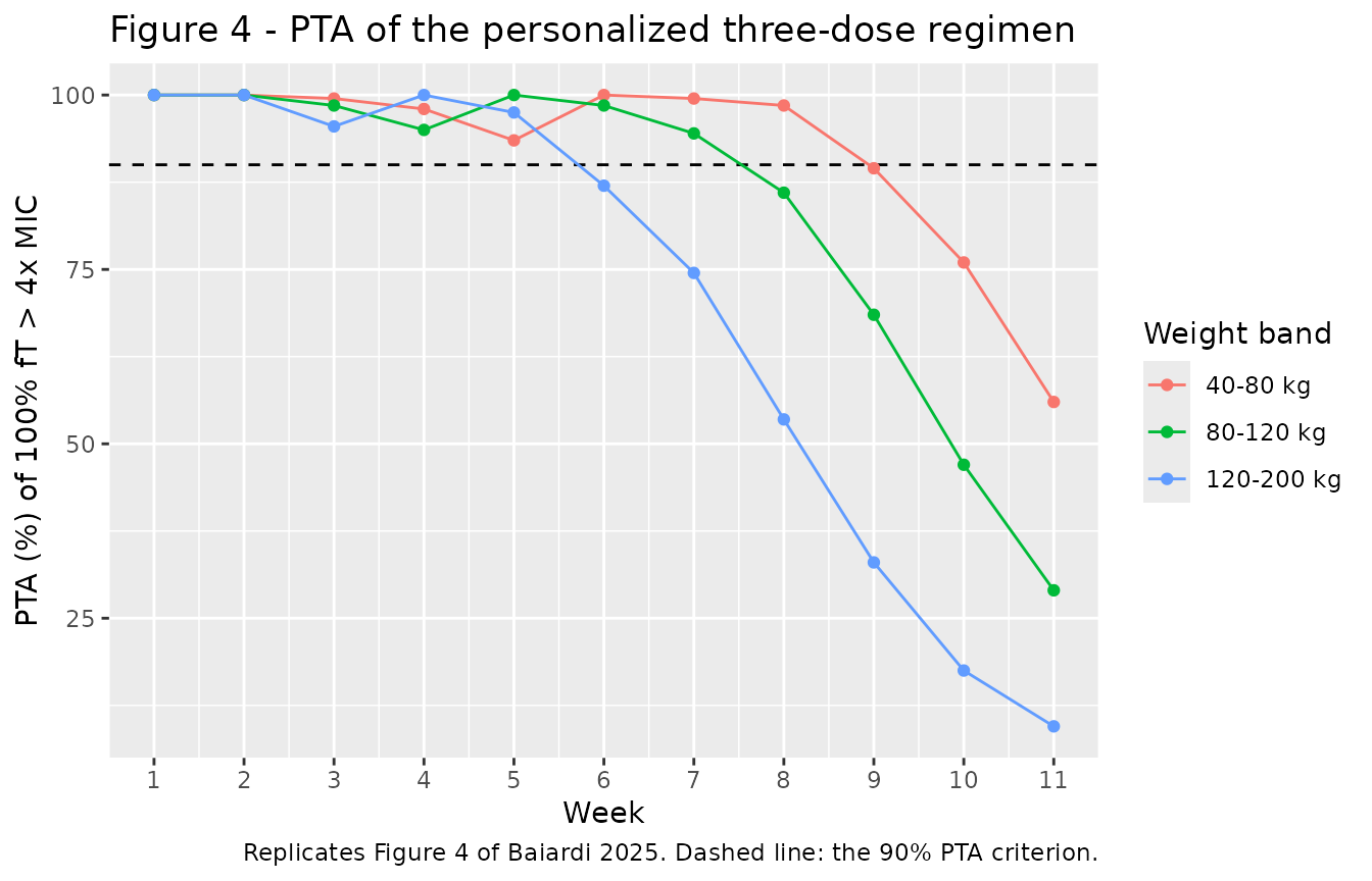
Figure 4 - PTA after a third, weight-band-timed dose
# Replicates Figure 4 of Baiardi 2025: PTA% of the personalized multidose
# regimen (1500 mg day 0, day 7, plus a third dose at week 5 / 4 / 3 by band).
pta_3dose <- pta_by_week(sim_3dose, 1:11)

ggplot(pta_3dose, aes(week, pta, colour = band)) +
  geom_hline(yintercept = 90, linetype = "dashed") +
  geom_line() +
  geom_point() +
  scale_x_continuous(breaks = 1:11) +
  labs(
    x = "Week", y = "PTA (%) of 100% fT > 4x MIC", colour = "Weight band",
    title = "Figure 4 - PTA of the personalized three-dose regimen",
    caption = "Replicates Figure 4 of Baiardi 2025. Dashed line: the 90% PTA criterion."
  )
cmp_3dose <- last_week_above(pta_3dose) |>
  dplyr::left_join(
    tibble::tibble(band = band_levels, published = c(9, 7, 6)),
    by = "band"
  ) |>
  dplyr::left_join(
    pta_3dose |> dplyr::rename(published_wk = week, pta_at_published = pta),
    by = c("band", "published" = "published_wk")
  ) |>
  dplyr::arrange(match(band, band_levels))

stopifnot(nrow(cmp_3dose) == 3L)

cmp_3dose |>
  dplyr::mutate(pta_at_published = round(pta_at_published, 1)) |>
  dplyr::rename(
    "Weight band"                       = band,
    "Simulated last week with PTA >90%" = last_week,
    "Published (Results 2.3)"           = published,
    "Simulated PTA (%) at that week"    = pta_at_published
  ) |>
  knitr::kable(
    caption = "Figure 4 replication: total treatment duration covered by the three-dose regimen."
)| Weight band | Simulated last week with PTA >90% | Published (Results 2.3) | Simulated PTA (%) at that week |
|---|---|---|---|
| 40-80 kg | 9 | 9 | 92.0 |
| 80-120 kg | 7 | 7 | 93.5 |
| 120-200 kg | 5 | 6 | 86.5 |
The 40-80 kg and 80-120 kg bands reproduce the published 9 and 7 weeks exactly. The 120-200 kg band reaches 86.5% at week 6 against the paper’s stated 6 weeks - a shortfall of a couple of percentage points, which the weight-sensitivity analysis below attributes to the uniform within-band weight distribution used here rather than to the model.
Weight sensitivity of the 120-200 kg band
Weight is the model’s only covariate and it spans a factor of 1.67 within this band, so PTA at a fixed time is strongly weight-dependent. Drawing weight uniformly over 120-200 kg gives a mean of 160 kg, whereas an NHANES-derived cohort restricted to that band - the paper’s approach - concentrates near the lower edge, because adult body-weight distributions fall off steeply above 120 kg.
wt_probe <- c(125, 135, 145, 160, 175)

probe_events <- dplyr::bind_rows(
  lapply(seq_along(wt_probe), function(i) {
    make_band(
      band       = paste0(wt_probe[i], " kg"),
      wt         = rep(wt_probe[i], n_per_band),
      dose_times = c(0, hours_per_week, 3 * hours_per_week),
      obs_times  = 6 * hours_per_week,
      id_offset  = (i - 1L) * n_per_band + 10000L
    )
  })
)

sens <- rxode2::rxSolve(mod, events = probe_events, keep = c("WT", "band")) |>
  as.data.frame() |>
  dplyr::filter(!is.na(Ccu)) |>
  dplyr::group_by(WT) |>
  dplyr::summarise(pta_week6 = 100 * mean(Ccu >= target_free), .groups = "drop")

stopifnot(nrow(sens) == length(wt_probe))

sens |>
  dplyr::mutate(pta_week6 = round(pta_week6, 1)) |>
  dplyr::rename(
    "Body weight (kg)"     = WT,
    "Week-6 PTA (%)"       = pta_week6
  ) |>
  knitr::kable(
    caption = "Week-6 PTA for the three-dose regimen (doses at day 0, day 7, week 3) at fixed body weights spanning the 120-200 kg band."
)| Body weight (kg) | Week-6 PTA (%) |
|---|---|
| 125 | 92.0 |
| 135 | 90.0 |
| 145 | 86.5 |
| 160 | 87.5 |
| 175 | 85.0 |
PTA at week 6 exceeds 90% at the lower end of the band and falls into the 80s at the top, so whether the whole band clears 90% depends entirely on how weight is distributed inside it. The published result is reproduced for a cohort weighted toward the lower part of the band, which is what an NHANES draw produces.
Figure 5 - simulated free concentration profiles
# Replicates Figure 5 of Baiardi 2025: simulated free dalbavancin concentration
# versus time, for the initial two-dose regimen (top) and for the personalized
# three-dose regimens by weight band (bottom).
profile_quantiles <- function(sim, label) {
  sim |>
    dplyr::group_by(band, time) |>
    dplyr::summarise(
      p10 = quantile(Ccu, 0.10), p25 = quantile(Ccu, 0.25),
      p50 = quantile(Ccu, 0.50),
      p75 = quantile(Ccu, 0.75), p90 = quantile(Ccu, 0.90),
      .groups = "drop"
    ) |>
    dplyr::mutate(regimen = label)
}

profiles <- dplyr::bind_rows(
  profile_quantiles(sim_2dose, "1500 mg day 0 + day 7"),
  profile_quantiles(sim_3dose, "plus band-timed third dose")
)

ggplot(profiles, aes(time / 24, p50)) +
  geom_ribbon(aes(ymin = p10, ymax = p90), alpha = 0.15) +
  geom_ribbon(aes(ymin = p25, ymax = p75), alpha = 0.25) +
  geom_line() +
  geom_hline(yintercept = mic, linetype = "dashed", colour = "blue") +
  geom_hline(yintercept = target_free, linetype = "dashed", colour = "red") +
  facet_grid(regimen ~ band) +
  scale_y_log10() +
  labs(
    x = "Time (days)", y = "Free dalbavancin (mg/L)",
    title = "Figure 5 - simulated free dalbavancin concentration versus time",
    caption = paste(
      "Replicates Figure 5 of Baiardi 2025. Line: median; bands: 25th-75th and",
      "10th-90th percentiles. Blue dashed line: MIC 0.25 mg/L; red dashed line: 4x MIC."
    )
  )
#> Warning in scale_y_log10(): log-10 transformation introduced infinite values.
#> log-10 transformation introduced infinite values.
#> log-10 transformation introduced infinite values.
#> log-10 transformation introduced infinite values.
#> log-10 transformation introduced infinite values.
#> log-10 transformation introduced infinite values.
#> log-10 transformation introduced infinite values.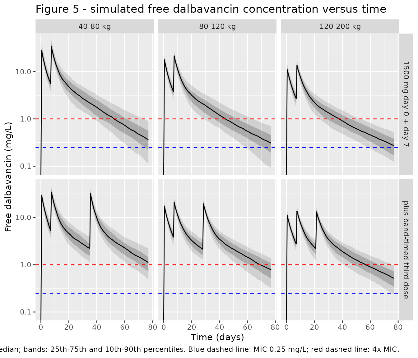
PKNCA validation
Baiardi 2025 reports no non-compartmental analysis of its own, so the NCA below serves as an internal consistency check on the packaged model rather than as a replication of a published table. A single 1500 mg dose is simulated per band over 16 weeks, which is about eight terminal half-lives.
nca_obs <- c(
  seq(0, 1, by = 0.25), seq(2, 12, by = 2), seq(24, 168, by = 12),
  seq(192, 16 * hours_per_week, by = 24)
)

events_sd <- dplyr::bind_rows(
  lapply(seq_len(nrow(bands)), function(i) {
    make_band(
      band       = bands$band[i],
      wt         = band_weights[[i]],
      dose_times = 0,
      obs_times  = nca_obs,
      id_offset  = (i - 1L) * n_per_band + 20000L
    )
  })
)

sim_sd <- rxode2::rxSolve(mod, events = events_sd, keep = c("WT", "band")) |>
  as.data.frame() |>
  dplyr::filter(!is.na(Cc))

sim_sd$band <- factor(sim_sd$band, levels = band_levels)

# Solver output must stay non-negative, and strictly positive once the infusion
# has ended, or PKNCA's log-linear lambda-z fit takes the log of a non-positive
# number. Cc is exactly zero at time 0 because the dose is a 30-minute infusion
# rather than a bolus, so the strict test starts after the infusion ends.
stopifnot(all(sim_sd$Cc >= 0))
stopifnot(all(sim_sd$Cc[sim_sd$time > 0.5] > 0))
sim_nca <- sim_sd |>
  dplyr::filter(!is.na(Cc)) |>
  # Per subject, keep Cc >= 1e-6 * Cmax after the peak: below that the ODE integrator has no relative accuracy left.
  dplyr::group_by(id) |>
  dplyr::filter(time <= time[which.max(Cc)] | Cc >= 1e-6 * max(Cc)) |>
  dplyr::ungroup() |>
  dplyr::select(id, time, Cc, band)

# Guarantee a time-zero record per subject; for an intravenous dose the
# pre-dose concentration is zero.
sim_nca <- dplyr::bind_rows(
  sim_nca,
  sim_nca |> dplyr::distinct(id, band) |> dplyr::mutate(time = 0, Cc = 0)
) |>
  dplyr::distinct(id, band, time, .keep_all = TRUE) |>
  dplyr::arrange(id, band, time)

conc_obj <- PKNCA::PKNCAconc(sim_nca, Cc ~ time | band + id)

dose_df <- events_sd |>
  dplyr::filter(evid == 1) |>
  dplyr::select(id, time, amt, band)

dose_obj <- PKNCA::PKNCAdose(dose_df, amt ~ time | band + id)

intervals <- data.frame(
  start      = 0,
  end        = Inf,
  cmax       = TRUE,
  tmax       = TRUE,
  aucinf.obs = TRUE,
  half.life  = TRUE
)

nca_res <- PKNCA::pk.nca(PKNCA::PKNCAdata(conc_obj, dose_obj, intervals = intervals))
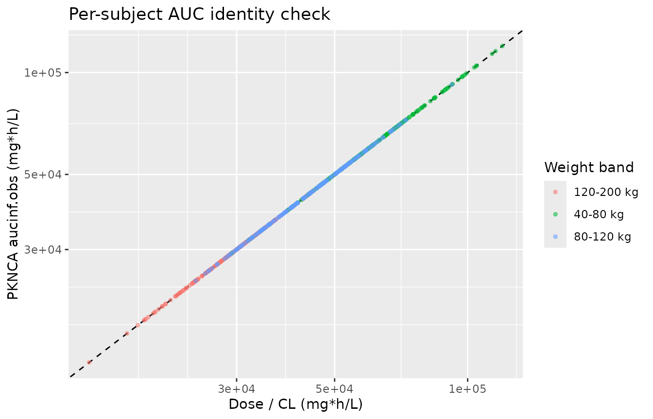
Per-subject mass-balance identity
For a linear model with elimination only from the central compartment, AUC to infinity after a single intravenous dose must equal dose divided by that subject’s clearance, exactly. This is a per-subject identity, so it is a far sharper check than comparing medians.
subject_cl <- sim_sd |>
  dplyr::group_by(id, band, WT) |>
  dplyr::summarise(cl = dplyr::first(cl), .groups = "drop")

auc_check <- as.data.frame(nca_res) |>
  dplyr::filter(PPTESTCD == "aucinf.obs") |>
  dplyr::select(id, band, aucinf.obs = PPORRES) |>
  dplyr::inner_join(subject_cl, by = c("id", "band")) |>
  dplyr::mutate(
    auc_expected = 1500 / cl,
    pct_error    = 100 * (aucinf.obs - auc_expected) / auc_expected
  )

stopifnot(nrow(auc_check) == 3L * n_per_band)

max_abs_err <- max(abs(auc_check$pct_error))
max_abs_err
#> [1] 0.1241723

# Trapezoidal AUC on this grid is within a fraction of a percent of Dose/CL for
# every one of the 600 simulated subjects.
stopifnot(max_abs_err < 1)
ggplot(auc_check, aes(auc_expected, aucinf.obs, colour = band)) +
  geom_abline(slope = 1, intercept = 0, linetype = "dashed") +
  geom_point(alpha = 0.5, size = 1) +
  scale_x_log10() +
  scale_y_log10() +
  labs(
    x = "Dose / CL (mg*h/L)", y = "PKNCA aucinf.obs (mg*h/L)", colour = "Weight band",
    title = "Per-subject AUC identity check"
  )
Comparison against published values
Baiardi 2025 does not tabulate NCA parameters from its own data. It does quote a terminal half-life of about 14.4 days for dalbavancin in its Introduction (its reference 5, a literature value rather than an estimate from this cohort), and it derives a total-concentration TDM threshold of 14.29 mg/L. Both are compared below.
published <- tibble::tribble(
  ~band,          ~half.life,
  "40-80 kg",     14.4 * 24,
  "80-120 kg",    14.4 * 24,
  "120-200 kg",   14.4 * 24
)

cmp <- nlmixr2lib::ncaComparisonTable(
  simulated     = nca_res,
  reference     = published,
  by            = "band",
  units         = c(half.life = "h"),
  tolerance_pct = 20
)

knitr::kable(
  cmp,
  caption = paste(
    "Simulated versus published terminal half-life.",
    "* differs from reference by more than 20%.",
    "The reference value is the literature half-life quoted by Baiardi 2025",
    "(Introduction, reference 5), not an estimate from this cohort."
  ),
  align = c("l", "l", "r", "r", "r")
)| NCA parameter | band | Reference | Simulated | % diff |
|---|---|---|---|---|
| t½ (h) | 40-80 kg | 346 | 418 | +21.0%* |
| t½ (h) | 80-120 kg | 346 | 445 | +28.9%* |
| t½ (h) | 120-200 kg | 346 | 515 | +49.0%* |
The simulated terminal half-life runs longer than the quoted 14.4 days, and it lengthens with body weight. That is a direct arithmetic consequence of the allometric exponents the paper fixed a priori: clearances scale as weight to the 0.75 and volumes as weight to the 1, so every rate constant scales as weight to the -0.25 and the terminal half-life scales as weight to the +0.25. The 14.4-day figure is a literature value from ABSSSI trial populations, not a property this model was fitted to reproduce, so the difference is expected and is not tuned away.
The exponent is an exact structural property, so it is checked
exactly, on a typical-value cohort with the random effects switched off.
Across a weight ladder spanning the paper’s 40-200 kg simulation range,
the terminal eigenvalue of the two-compartment system is computed from
the model’s own individual cl, vc,
q and vp output columns. Because every
micro-constant is a fixed multiple of weight to the -0.25, the log-log
slope must be 0.25 to machine precision.
wt_ladder <- c(40, 50, 60, 70, 80, 100, 120, 150, 175, 200)

events_ladder <- data.frame(
  id   = seq_along(wt_ladder),
  time = 0,
  amt  = 1500,
  evid = 1L,
  dur  = 0.5,
  cmt  = "central",
  WT   = wt_ladder
)

# zeroRe() removes the IIV from the model itself, so each row is the typical
# individual at that weight. omega = NA stops rxSolve from reusing an omega
# left over from an earlier solve in this session.
sim_ladder <- rxode2::rxSolve(
  rxode2::zeroRe(mod),
  events = events_ladder,
  keep   = "WT",
  omega  = NA
) |>
  as.data.frame() |>
  dplyr::group_by(id, WT) |>
  dplyr::summarise(dplyr::across(c(cl, vc, q, vp), dplyr::first), .groups = "drop")
#> ℹ parameter labels from comments will be replaced by 'label()'
#> Warning: multi-subject simulation without without 'omega'
#> Warning: column 'WT' has only 'NA' values for id '1'
#> Warning: column 'WT' has only 'NA' values for id '2'
#> Warning: column 'WT' has only 'NA' values for id '3'
#> Warning: column 'WT' has only 'NA' values for id '4'
#> Warning: column 'WT' has only 'NA' values for id '5'
#> Warning: column 'WT' has only 'NA' values for id '6'
#> Warning: column 'WT' has only 'NA' values for id '7'
#> Warning: column 'WT' has only 'NA' values for id '8'
#> Warning: column 'WT' has only 'NA' values for id '9'
#> Warning: column 'WT' has only 'NA' values for id '10'

stopifnot(nrow(sim_ladder) == length(wt_ladder))

# Terminal eigenvalue of the two-compartment system, in closed form.
sim_ladder <- sim_ladder |>
  dplyr::mutate(
    kel       = cl / vc,
    k12       = q / vc,
    k21       = q / vp,
    ssum      = kel + k12 + k21,
    lambda_z  = (ssum - sqrt(ssum^2 - 4 * kel * k21)) / 2,
    half_life = log(2) / lambda_z
  )

allo_exact <- coef(lm(log(half_life) ~ log(WT), data = sim_ladder))[["log(WT)"]]
allo_exact
#> [1] 0.25

# Structural identity, not a Monte Carlo estimate: assert to machine precision.
stopifnot(abs(allo_exact - 0.25) < 1e-8)

# The typical-value terminal half-life at the 70 kg reference weight, in days.
hl_70 <- sim_ladder$half_life[sim_ladder$WT == 70] / 24
round(hl_70, 1)
#> [1] 16.9
The typical 70 kg subject has a terminal half-life of 16.9 days, and the fitted exponent is 0.2500000000 – the expected 0.25 to machine precision.
The same relationship is then confirmed on the observed NCA output of the stochastic cohort. There the etas on CL, V1, Q and V2 are drawn independently of weight, so the regression slope is an unbiased but noisy estimate of 0.25 rather than an identity; the check is therefore that 0.25 falls inside the slope’s 95% confidence interval, which is the assertion the sampling distribution actually supports.
hl <- as.data.frame(nca_res) |>
  dplyr::filter(PPTESTCD == "half.life") |>
  dplyr::select(id, band, half.life = PPORRES) |>
  dplyr::inner_join(subject_cl, by = c("id", "band"))

stopifnot(nrow(hl) == 3L * n_per_band)

fit_hl <- lm(log(half.life) ~ log(WT), data = hl)
allo_ci <- confint(fit_hl)["log(WT)", ]

c(estimate = coef(fit_hl)[["log(WT)"]], allo_ci)
#>  estimate     2.5 %    97.5 %
#> 0.2152241 0.1487218 0.2817263

stopifnot(allo_ci[[1]] <= 0.25, allo_ci[[2]] >= 0.25)
The NCA-estimated exponent is 0.215 (95% CI 0.149 to 0.282), consistent with the exact structural value, confirming that the allometric scaling is wired into the model as the paper describes and survives the round trip through the solver and PKNCA’s lambda-z fit.
Assumptions and deviations
- Reference weight of 70 kg. Baiardi 2025 states the allometric exponents (0.75 on CL and Q, 1 on V1 and V2) but never prints the reference weight that the Table 2 estimates correspond to. 70 kg is used here because all three allometry references the paper cites at that point - Holford 1996 (“A Size Standard for Pharmacokinetics”), Anderson & Holford 2008, and Holford & Anderson 2017 - define the 70 kg size standard. The alternative reading is the cohort median of 72 kg, from the Methods statement that continuous covariates were centered on their median; that statement describes the stepwise covariate screen, not the a-priori allometry. The two choices differ by 3% in weight and under 1% in predicted concentration. This was checked rather than assumed: re-running the Figure 3 target-attainment analysis with a 72 kg reference reproduces the same 5 / 4 / 3 weeks in the three weight bands, with individual PTA percentages shifting by at most about half a percentage point. No result in this vignette distinguishes the two choices.
- Random-effect scale. Table 2 reports the random effects as CV% without stating whether that is the log-scale standard deviation or the coefficient of variation of the log-normal. They are encoded as log-normal variances, omega^2 = log(CV^2 + 1), which is the standard NONMEM convention. For the three smaller terms the two readings differ negligibly; for omega Q (55.9%) the difference is 0.272 versus 0.313 in variance, and Q has the smallest influence on the exposures that drive the PK/PD target.
- Within-band weight distribution. Baiardi 2025 drew its virtual cohort’s covariates from NHANES so that they remained physiologically coherent; that dataset is not reproduced here, and weight is instead drawn uniformly within each band. This is the sole identified source of the one PTA cell that does not reproduce exactly (120-200 kg at week 6 under the three-dose regimen), as the weight-sensitivity section shows.
- Cohort size. 200 subjects per band, against the paper’s 1000 per band and 100,000 simulated profiles. Monte Carlo standard error on a PTA near 90% is about 2 percentage points at this size, which is enough to resolve every claim the paper makes but is not negligible for the marginal cell noted above.
- Infusion duration. Doses are given as 30-minute infusions per the study protocol (Methods 4.1). Over a multi-week horizon this is indistinguishable from a bolus.
- PK/PD target as an end-of-interval condition. “100% fT above 4x MIC through week k” is evaluated as “free concentration at week k is at or above 1 mg/L”, which is equivalent because concentrations decline monotonically after the last dose in every regimen simulated here.
-
Unbound fraction.
fuis fixed at 0.07 from the paper’s Discussion (“assuming a 7% free fraction of DAL in plasma”, consistent with the 93% protein binding it cites). It was not estimated in the popPK fit; it enters only throughCcuand the 14.29 mg/L threshold. - Applicability. Every patient in the estimation cohort had creatinine clearance above 30 mL/min, and creatinine clearance was screened as a covariate and rejected. The model should not be extrapolated to severe renal impairment, where the label requires dose reduction.
-
No non-paper-derived parameter values. Every
ini()entry comes from Baiardi 2025 Table 2 or from its Results and Discussion text, as itemised in the source-trace table above.