Ceftaroline (Riccobene 2016)

Model and source

• Citation: Riccobene TA, Pushkin R, Jandourek A, Knebel W, Khariton T. Penetration of ceftaroline into the epithelial lining fluid of healthy adult subjects. Antimicrob Agents Chemother. 2016;60(10):5849-5857. doi:10.1128/AAC.02755-15. Parameter estimates are from Supplemental Table 1 and the model equations from Supplemental Equation 1 of that article’s supplemental material. Structural model and the fixed covariate effects were carried from the upstream adult ceftaroline fosamil / ceftaroline population PK analysis of 10 phase 1, 1 phase 2 and 4 phase 3 studies cited as reference 14 of Riccobene 2016 (Riccobene T, Khariton T, Knebel W, O’Neal T, Ghahramani P. 2013. Abstr 23rd Eur Congr Clin Microbiol Infect Dis, abstr P902); that abstract is not in nlmixr2lib.
• Article: https://doi.org/10.1128/AAC.02755-15
• Supplement (Supplemental Table 1 = final parameter estimates; Supplemental Equation 1 = structural model): https://doi.org/10.1128/AAC.02755-15 (supplemental material, file zac010165525so1)

Ceftaroline fosamil is a water-soluble N-phosphono prodrug that systemic phosphatases convert rapidly to ceftaroline, the active anti-MRSA cephalosporin. Riccobene 2016 measured ceftaroline in plasma and in bronchoalveolar-lavage epithelial lining fluid (ELF) at steady state in healthy adults and fitted a joint population PK model to both matrices, in order to run PK/PD target attainment simulations for MRSA pneumonia.

The packaged model carries three analyte layers:

• ceftaroline fosamil (the dosed prodrug) as a two-compartment system, in the canonical unsuffixed central / peripheral1 states;
• ceftaroline (the active metabolite) as a three-compartment system in central_ceftaroline / peripheral1_ceftaroline / peripheral2_ceftaroline, formed by the whole prodrug elimination clearance CLcf;
• ELF as an algebraic scaling of the ceftaroline plasma concentration by a partition coefficient, not as a distribution compartment. Plasma and ELF declined in parallel (paper Figure 1), so an ELF compartment was not identifiable.

Population

Fifty healthy adults completed a single-centre, phase 1, open-label, multiple-dose study (Pulmonary Associates, Phoenix, AZ) and contributed to the population PK analysis: 25 given 600 mg ceftaroline fosamil as a 1-h IV infusion every 12 h and 25 given the same dose every 8 h, each for 3 days plus a single dose on day 4. Of the 53 subjects enrolled (paper Table 1), 69.2% / 92.6% were White in the q12h / q8h arms and 92.3% / 70.4% were male; mean age was 34.6 and 33.1 years. The 50-subject analysis population was 42 males and 8 females, aged 20 to 45 years and weighing 58 to 102 kg (Results, “Population pharmacokinetics in the lung”). Subjects were nonsmokers with a body mass index of 18 to 30 kg/m^2 and no clinically significant disease.

That cohort composition is what makes several of the model’s covariate effects uninformed by these data: nobody had end-stage renal disease, nobody was dialysed, nobody had a BSA-normalised creatinine clearance below 80 mL/min/1.73 m^2 and nobody was over 45 years old (Methods, “Population pharmacokinetics in the lung”). Those coefficients were therefore fixed to the values of the upstream pooled adult analysis of 10 phase 1, 1 phase 2 and 4 phase 3 studies, and are carried here as fixed().

Plasma sampling on day 4 was dense (14 time points from predose to 24 h), but each subject underwent bronchoalveolar lavage at exactly one of five post-dose times (five subjects per time point), so the published ELF profile is a sparse composite of medians across subjects rather than a set of individual profiles. 856 plasma concentrations (210 ceftaroline fosamil, 646 ceftaroline) and 49 ELF concentrations (43 of them ceftaroline) entered the fit.

The same information is available programmatically:

readModelDb("Riccobene_2016_ceftaroline")()$population[
  c("species", "n_subjects", "age_range", "weight_range", "dose_range")
]
#> $species
#> [1] "human"
#> 
#> $n_subjects
#> [1] 50
#> 
#> $age_range
#> [1] "20-45 years (enrolled 19-45; mean 34.6 years in the q12h arm and 33.1 years in the q8h arm)"
#> 
#> $weight_range
#> [1] "58-102 kg"
#> 
#> $dose_range
#> [1] "600 mg ceftaroline fosamil as a 1-h IV infusion, q12h or q8h for 3 days plus a single dose on day 4"

Source trace

Every ini() entry in inst/modeldb/specificDrugs/Riccobene_2016_ceftaroline.R carries an in-file comment naming its source location. The table below collects them.

Supplemental Table 1 prints back-transformed values: Supplemental Equation 1 writes each structural parameter as exp(theta + log(WT/70) * exponent + eta), so the tabulated number is the typical value at the reference covariates rather than the log-scale theta. The variability section of the table reports variances, with the parenthetical %CV / SD columns being their square roots (e.g. propCF = 0.0658 variance, %CV = 25.7); the residual SDs below are therefore sqrt(variance).

Equation / parameter	Value	Source location
lcl (CLcf)	238 L/h (206, 274)	Suppl. Table 1, theta1
lvc (Vccf)	6.96 L, fixed	Suppl. Table 1, theta2
lq (Qcf)	97.4 L/h (57.3, 165)	Suppl. Table 1, theta3
lvp (Vpcf)	6.23 L (4.26, 9.1)	Suppl. Table 1, theta4
lka (kacf, IM only)	0.549 1/h, fixed	Suppl. Table 1, theta5
lfdepot (FIMcf)	1, fixed	Suppl. Table 1, theta6
lcl_ceftaroline (CLc)	3.76 L/h (3.6, 3.93)	Suppl. Table 1, theta7
lvc_ceftaroline (Vcc)	3.18 L (2.72, 3.73)	Suppl. Table 1, theta8
lq_ceftaroline (Q1c)	3.71 L/h (2.66, 5.19)	Suppl. Table 1, theta9
lvp_ceftaroline (Vp1c)	7.14 L (6.13, 8.32)	Suppl. Table 1, theta10
lq2_ceftaroline (Q2c)	18.6 L/h (13.7, 25.3)	Suppl. Table 1, theta18
lvp2_ceftaroline (Vp2c)	6.76 L (5.71, 8)	Suppl. Table 1, theta19
lcl_hemodialysis_ceftaroline (CLdial)	9.97 L/h, fixed	Suppl. Table 1, theta14
lrelf (PCELF)	0.193 (0.161, 0.226)	Suppl. Table 1, theta17; main text Results quotes (0.171, 0.215)
e_wt_cl_q	0.75, fixed	Suppl. Table 1, (WT/70)^0.75 rows
e_wt_vc_vp	1, fixed	Suppl. Table 1, (WT/70)^1 rows
e_crcl_cl_ceftaroline	0.508, fixed	Suppl. Table 1, theta11
e_age_cl_ceftaroline	-0.278, fixed	Suppl. Table 1, theta13
e_dis_healthy_cl_ceftaroline	3.32, fixed	Suppl. Table 1, theta16 (source PAT; re-expressed, see Errata)
e_dis_healthy_vc_ceftaroline	3.67, fixed	Suppl. Table 1, theta15 (source PAT; re-expressed, see Errata)
e_rrt_hemodial_status_cl_ceftaroline	0.372, fixed	Suppl. Table 1, theta12 (source ESRD)
IIV block (CLcf, Vccf, CLc, Vcc)	4x4 lower triangle	Suppl. Table 1, “Inter-individual variability”
etalvp_ceftaroline	0.02 (%CV 14.1)	Suppl. Table 1, VAR(Vp1c)
etalrelf	0.128 (%CV 35.8)	Suppl. Table 1, VAR(PCELF)
propSd / addSd	0.2565 / 0.0487 mg/L	Suppl. Table 1, propCF 0.0658 / addCF 0.00237
propSd_ceftaroline / addSd_ceftaroline	0.0528 / 0.102 mg/L	Suppl. Table 1, propC 0.00279 / addC 0.0105
propSd_Celf	0.0632, fixed	Suppl. Table 1, propELF 0.004
Prodrug and metabolite ODEs, complete conversion	n/a	Suppl. Equation 1, CLcf/Vccf/Q1cf/Vp1cf and Vcc/Qc/Vpc/CLc blocks
ELF as Cc_ceftaroline * PC	n/a	Suppl. Equation 1, lines “PC = theta17 * exp(etaPC)” and “Cij = Chat_ij * PC + Chat_ij * PC * eps_p3ij”
Renal-function gate below 80 mL/min/1.73 m^2	n/a	Suppl. Equation 1, COV3; main text Results
Dialysis-session clearance replacement	n/a	Suppl. Equation 1, “for dialysis patients during dialysis, CLc_i = exp(theta14)”

Virtual cohort

The observed data are not public, so the simulations use virtual cohorts whose covariates span the published ranges. Covariates are placed on a deterministic quantile grid rather than drawn at random, so the vignette’s numbers are reproducible and are not hostage to a lucky or unlucky draw.

n_per_arm <- 200L
tau_q12h <- 12
tau_q8h <- 8

# Deterministic quantile grid, clamped to the observed ranges reported in
# Results ("Population pharmacokinetics in the lung"): WT 58-102 kg,
# AGE 20-45 y. The normal parameters are chosen so the central 95% of the
# distribution spans the reported range.
quantile_grid <- function(n, mean, sd, lo, hi) {
  p <- (seq_len(n) - 0.5) / n
  pmin(pmax(qnorm(p, mean, sd), lo), hi)
}

make_arm <- function(n, tau, label, id_offset) {
  # Built here, not inside crossing(): inside the data mask `tau` would resolve
  # to the per-subject column rather than the scalar interval. 1.0833 h is the
  # 65-min post-infusion sample of the paper's day-4 schedule.
  tgrid <- sort(unique(c(seq(0, tau, by = 0.25), 1, 1.0833)))

  covs <- tibble(
    id = id_offset + seq_len(n),
    WT = quantile_grid(n, 80, 11.2, 58, 102),
    # AGE is reversed against WT so the two are not perfectly rank-correlated.
    AGE = rev(quantile_grid(n, 34, 6.6, 20, 45)),
    # All subjects were healthy with normal renal function and none were
    # dialysed. CRCL enters only through min(CRCL, 80), so any value at or
    # above 80 leaves the renal term at exactly 1.
    CRCL = 100,
    DIS_HEALTHY = 1,
    RRT_HEMODIAL_STATUS = 0,
    RRT_HEMODIAL_ACTIVE = 0,
    treatment = label,
    tau = tau
  )

  # Steady state on day 4 is imposed with ss = 1 / ii = tau rather than by
  # dosing forward from zero, so the profile is the converged interval the
  # paper sampled. dur = 1 encodes the 1-h IV infusion.
  doses <- covs |>
    mutate(time = 0, amt = 600, dur = 1, evid = 1L, ii = tau, ss = 1L,
           cmt = "central", dvid = NA_integer_)

  # Observation rows carry dvid, not a compartment name: the model declares
  # three endpoints (Cc, Cc_ceftaroline, Celf), so rxode2 requires the dvid
  # -> endpoint mapping on observation records. rxSolve returns all three
  # observables as columns at every observation row regardless of which dvid
  # is requested, so one dvid is enough.
  obs <- covs |>
    tidyr::crossing(time = tgrid) |>
    mutate(amt = NA_real_, dur = NA_real_, evid = 0L, ii = 0, ss = 0L,
           cmt = NA_character_, dvid = 2L)

  bind_rows(doses, obs) |> arrange(id, time, desc(evid))
}

events <- bind_rows(
  make_arm(n_per_arm, tau_q12h, "600 mg q12h", 0L),
  make_arm(n_per_arm, tau_q8h, "600 mg q8h", n_per_arm)
)

# Disjoint ids across arms are mandatory: rxSolve keys subjects on id alone,
# so a shared id would silently merge the two regimens into one subject.
stopifnot(!anyDuplicated(unique(events[, c("id", "time", "evid")])))
stopifnot(length(unique(events$id)) == 2L * n_per_arm)

Simulation

mod <- readModelDb("Riccobene_2016_ceftaroline")

# useLinCmt = FALSE: rxode2's automatic ODE -> linCmt() conversion corrupts the
# dvid -> cmt mapping for multi-output models of this shape.
sim <- rxode2::rxSolve(
  mod,
  events = events,
  keep = c("treatment", "tau", "WT", "AGE"),
  useLinCmt = FALSE
) |>
  as.data.frame()
#> ℹ parameter labels from comments will be replaced by 'label()'

# Typical-value profiles for the figure replications. omega = NA zeroes the
# random effects for this solve only; zeroRe() would mutate the shared model
# object and silently strip IIV from every later chunk.
sim_typical <- rxode2::rxSolve(
  mod,
  events = events |> filter(id %in% c(1L, n_per_arm + 1L)) |>
    mutate(WT = 80, AGE = 34),
  keep = c("treatment", "tau"),
  omega = NA,
  useLinCmt = FALSE
) |>
  as.data.frame()
#> Warning: multi-subject simulation without without 'omega'

nrow(sim)
#> [1] 16800

Replicate published figures

Figure 1 - plasma and ELF ceftaroline at steady state

Paper Figure 1 plots mean ceftaroline concentrations in plasma and ELF after the last day-4 dose for both regimens; paper Table 3 tabulates the medians that the figure draws. The typical-value curves below are overlaid on those tabulated medians.

# Paper Table 3, "Plasma and ELF concentrations of ceftaroline in healthy
# subjects" -- median total plasma and median ELF at each sampled time.
observed <- tibble::tribble(
  ~treatment,     ~time, ~plasma, ~elf,
  "600 mg q12h",   1,     18.73,  3.38,
  "600 mg q12h",   2,      8.47,  1.60,
  "600 mg q12h",   4,      3.27,  0.54,
  "600 mg q12h",   8,      0.90,  0.18,
  "600 mg q12h",  12,      0.27,  0.00,
  "600 mg q8h",    1,     21.31,  3.56,
  "600 mg q8h",    2,      9.46,  2.57,
  "600 mg q8h",    4,      3.56,  0.58,
  "600 mg q8h",    6,      1.74,  0.27,
  "600 mg q8h",    8,      0.99,  0.26
)

pred_long <- sim_typical |>
  filter(!is.na(Cc_ceftaroline)) |>
  select(treatment, time, plasma = Cc_ceftaroline, elf = Celf) |>
  pivot_longer(c(plasma, elf), names_to = "matrix", values_to = "conc")

obs_long <- observed |>
  pivot_longer(c(plasma, elf), names_to = "matrix", values_to = "conc") |>
  filter(conc > 0)

ggplot(pred_long, aes(time, conc, colour = matrix)) +
  geom_line(linewidth = 0.8) +
  geom_point(data = obs_long, aes(shape = matrix), size = 2.4) +
  facet_wrap(~treatment, scales = "free_x") +
  scale_y_log10() +
  labs(x = "Time after the last dose (h)", y = "Ceftaroline (mg/L)",
       colour = "Matrix", shape = "Matrix",
       title = "Figure 1 - plasma and ELF ceftaroline at steady state",
       caption = "Replicates Figure 1 of Riccobene 2016.")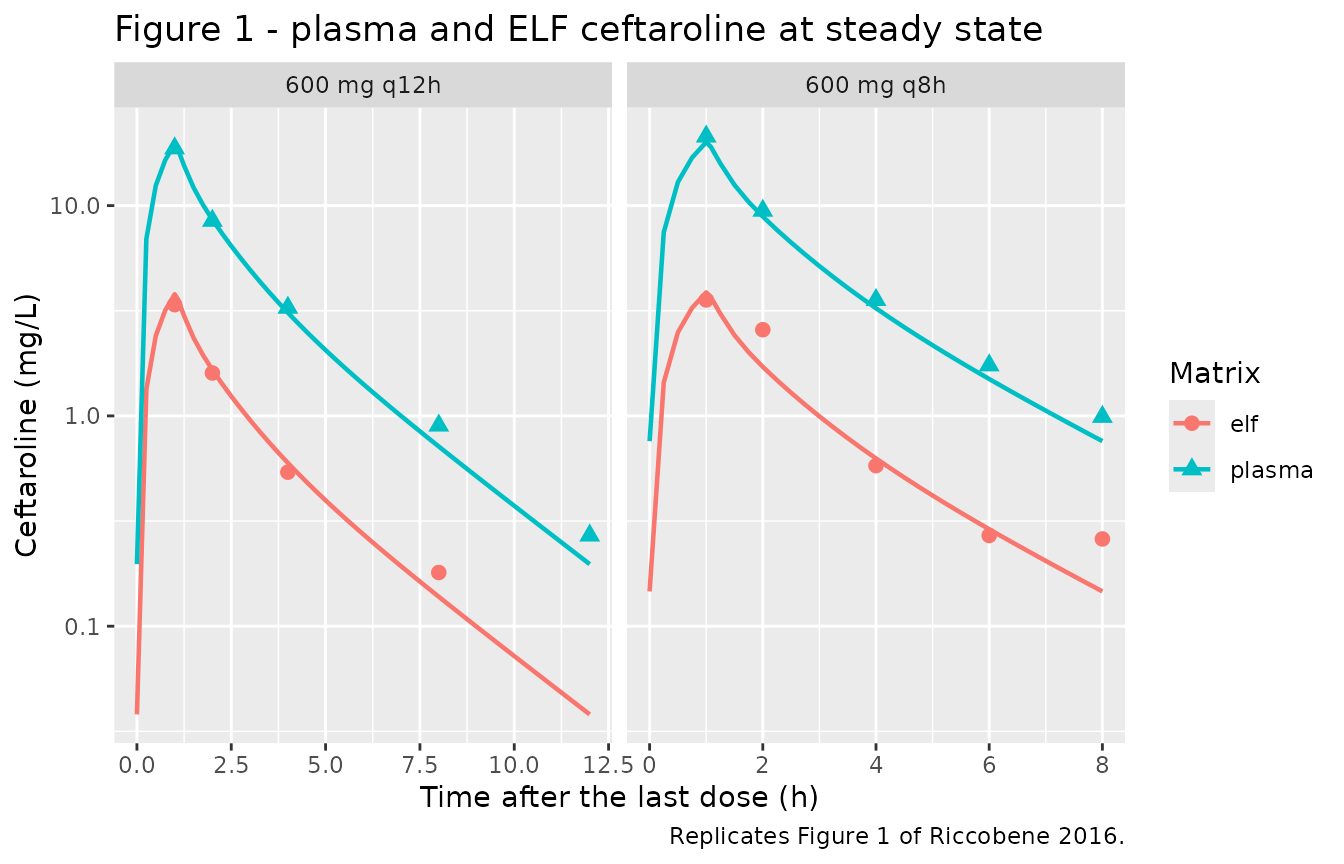

Replicates Figure 1 of Riccobene 2016. Lines are typical-value predictions from the packaged model; points are the published medians of Table 3.

# Strict point-by-point comparison against every median in Table 3.
t3 <- observed |>
  pivot_longer(c(plasma, elf), names_to = "matrix", values_to = "observed") |>
  filter(observed > 0) |>
  left_join(
    sim_typical |>
      filter(!is.na(Cc_ceftaroline)) |>
      select(treatment, time, plasma = Cc_ceftaroline, elf = Celf) |>
      pivot_longer(c(plasma, elf), names_to = "matrix", values_to = "predicted"),
    by = c("treatment", "time", "matrix")
  ) |>
  mutate(`Ratio pred/obs` = round(predicted / observed, 2))

t3 |>
  mutate(across(c(observed, predicted), ~ round(.x, 2))) |>
  rename("Regimen" = treatment, "Time (h)" = time, "Matrix" = matrix,
         "Published median (mg/L)" = observed,
         "Model typical (mg/L)" = predicted) |>
  knitr::kable(caption = "Model typical values vs the published medians of Riccobene 2016 Table 3.")

Model typical values vs the published medians of Riccobene 2016 Table 3.

Regimen	Time (h)	Matrix	Published median (mg/L)	Model typical (mg/L)	Ratio pred/obs
600 mg q12h	1	plasma	18.73	19.63	1.05
600 mg q12h	1	elf	3.38	3.79	1.12
600 mg q12h	2	plasma	8.47	8.58	1.01
600 mg q12h	2	elf	1.60	1.66	1.03
600 mg q12h	4	plasma	3.27	3.10	0.95
600 mg q12h	4	elf	0.54	0.60	1.11
600 mg q12h	8	plasma	0.90	0.72	0.79
600 mg q12h	8	elf	0.18	0.14	0.77
600 mg q12h	12	plasma	0.27	0.20	0.73
600 mg q8h	1	plasma	21.31	20.04	0.94
600 mg q8h	1	elf	3.56	3.87	1.09
600 mg q8h	2	plasma	9.46	8.87	0.94
600 mg q8h	2	elf	2.57	1.71	0.67
600 mg q8h	4	plasma	3.56	3.25	0.91
600 mg q8h	4	elf	0.58	0.63	1.08
600 mg q8h	6	plasma	1.74	1.50	0.86
600 mg q8h	6	elf	0.27	0.29	1.07
600 mg q8h	8	plasma	0.99	0.76	0.77
600 mg q8h	8	elf	0.26	0.15	0.56

# The prediction should track the published medians within a factor of two at
# every sampled time in both matrices and both regimens.
stopifnot(all(t3$`Ratio pred/obs` > 0.5 & t3$`Ratio pred/obs` < 2))

Supplemental Figure 1 - ceftaroline fosamil in plasma

The prodrug is cleared so fast that the paper could not compute NCA parameters for it (“PK parameters therefore could not be determined for the prodrug ceftaroline fosamil”), so there is no published table to compare against. What Supplemental Figure 1 does pin down is the axis scale and shape: a 0 to 4 h time axis, a 0 to 4 mg/L linear concentration axis in panel A with the peak at the end of the 1-h infusion, and a semilogarithmic panel B spanning 0.001 to 10 mg/L over which the curve falls away well before 4 h. The checks below assert only those figure-supported bounds; the peak height itself is reported rather than asserted, because it cannot be read off the published figure precisely.

sim_typical |>
  filter(!is.na(Cc), Cc > 0, time <= 4) |>
  ggplot(aes(time, Cc, colour = treatment)) +
  geom_line(linewidth = 0.8) +
  scale_y_log10(limits = c(1e-3, 10)) +
  labs(x = "Time after the last dose (h)",
       y = "Ceftaroline fosamil (mg/L)", colour = "Regimen",
       title = "Supplemental Figure 1 - ceftaroline fosamil in plasma",
       caption = "Replicates Supplemental Figure 1 of Riccobene 2016.")
#> Warning: Removed 20 rows containing missing values or values outside the scale range
#> (`geom_line()`).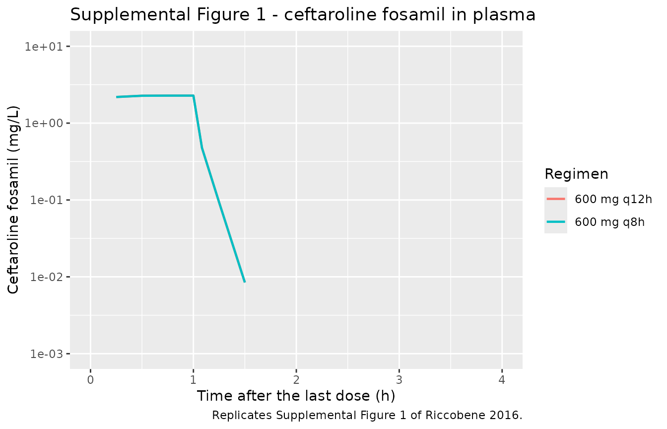

Replicates Supplemental Figure 1 of Riccobene 2016 (semilogarithmic panel B).

fos <- sim_typical |> filter(!is.na(Cc))
fos_summary <- fos |>
  group_by(treatment) |>
  summarise(`Peak (mg/L)` = round(max(Cc), 2),
            `Time of peak (h)` = time[which.max(Cc)],
            `Concentration at 4 h (mg/L)` = round(max(Cc[abs(time - 4) < 1e-8], 0), 5),
            .groups = "drop")
knitr::kable(fos_summary,
             caption = "Ceftaroline fosamil typical-value profile; compare with Supplemental Figure 1 of Riccobene 2016.")

Ceftaroline fosamil typical-value profile; compare with Supplemental Figure 1 of Riccobene 2016.

treatment	Peak (mg/L)	Time of peak (h)	Concentration at 4 h (mg/L)
600 mg q12h	2.28	1	0
600 mg q8h	2.28	1	0

# Bounds that Supplemental Figure 1 actually supports: the peak is at the end of
# the 1-h infusion and lies inside panel A's 0-4 mg/L axis, and by 4 h the curve
# has dropped below the 0.01 mg/L gridline of the semilogarithmic panel B.
stopifnot(all(fos_summary$`Peak (mg/L)` > 0 & fos_summary$`Peak (mg/L)` < 4))
stopifnot(all(abs(fos_summary$`Time of peak (h)` - 1) < 1e-6))
stopifnot(all(fos_summary$`Concentration at 4 h (mg/L)` < 0.01))

PKNCA validation

Plasma ceftaroline

Paper Table 2 reports plasma NCA per subject over the day-4 dosing interval, so the simulated cohort is run through the same estimator: Cmax, tmax, terminal half-life and AUC0-tau over the steady-state interval. Following the paper, NCA is computed on the observed scale, so the simulated concentrations include residual error (sim rather than the IPRED-only typical solve).

Every observation row requested dvid = 2 (the Cc_ceftaroline endpoint), so rxode2’s sim column is the ceftaroline plasma concentration with residual error, while Cc_ceftaroline is the IPRED. Following the paper, concentrations below the assay’s lower limit of quantification for ceftaroline in plasma (50 ng/mL) are set to zero: “Concentrations below the limit of quantification were treated as 0 for all noncompartmental PK calculations.”

lloq_plasma <- 0.05   # mg/L; paper Methods, "Drug concentration in plasma"

# Only !is.na() -- a time > 0 or Cc > 0 filter would drop the time-zero row
# that anchors AUC0-tau and would trigger PKNCA's "AUC range starting before
# the first measurement" warning on every subject.
conc_plasma <- sim |>
  filter(!is.na(sim)) |>
  mutate(Cc_obs = if_else(sim < lloq_plasma, 0, sim)) |>
  select(id, time, treatment, tau, Cc_obs)

# Defensive time-zero guarantee. At steady state the predose concentration is
# the trough, which the ss = 1 solve already returns at time 0.
stopifnot(all(table(conc_plasma$id[conc_plasma$time == 0]) == 1))

conc_obj <- PKNCA::PKNCAconc(
  as.data.frame(conc_plasma), Cc_obs ~ time | treatment + id
)

dose_plasma <- events |>
  filter(evid == 1) |>
  select(id, time, amt, dur, treatment)

dose_obj <- PKNCA::PKNCAdose(
  as.data.frame(dose_plasma), amt ~ time | treatment + id,
  duration = "dur"
)

# One interval per regimen: 0 to tau of the steady-state interval.
intervals <- data.frame(
  start = 0,
  end = c(tau_q12h, tau_q8h),
  cmax = TRUE, tmax = TRUE, cmin = TRUE,
  auclast = TRUE, half.life = TRUE
)

nca_res <- PKNCA::pk.nca(
  PKNCA::PKNCAdata(conc_obj, dose_obj, intervals = intervals)
)

# PKNCA emits dependency rows (parameters computed only to support another
# parameter); filter on the interval bounds as well as the parameter name so
# results from the q12h and q8h intervals are not averaged together.
nca_plasma <- as.data.frame(nca_res) |>
  filter(PPTESTCD %in% c("cmax", "tmax", "half.life", "auclast")) |>
  mutate(tau_expected = if_else(treatment == "600 mg q12h", tau_q12h, tau_q8h)) |>
  filter(start == 0, end == tau_expected)

nca_plasma |>
  group_by(treatment, PPTESTCD) |>
  summarise(median = median(PPORRES), .groups = "drop") |>
  pivot_wider(names_from = PPTESTCD, values_from = median) |>
  mutate(across(where(is.numeric), ~ round(.x, 2))) |>
  knitr::kable(caption = "Simulated plasma ceftaroline NCA (medians over the virtual cohort).")

Simulated plasma ceftaroline NCA (medians over the virtual cohort).

treatment	auclast	cmax	half.life	tmax
600 mg q12h	42.36	19.27	NA	1
600 mg q8h	43.12	20.07	NA	1

# Paper Table 2, plasma column (mean +/- SD, n = 25 per arm).
published_plasma <- tibble::tribble(
  ~treatment,     ~cmax, ~tmax, ~half.life, ~auclast,
  "600 mg q12h",  19.7,  1.0,   2.41,       45.0,
  "600 mg q8h",   22.3,  1.0,   2.48,       53.0
)

cmp_plasma <- nlmixr2lib::ncaComparisonTable(
  simulated = nca_res,
  reference = published_plasma,
  by = "treatment",
  units = c(cmax = "mg/L", tmax = "h", half.life = "h", auclast = "mg*h/L"),
  tolerance_pct = 20
)

knitr::kable(
  cmp_plasma,
  caption = "Plasma ceftaroline: simulated vs Riccobene 2016 Table 2. * differs from reference by >20%.",
  align = c("l", "l", "r", "r", "r")
)

Plasma ceftaroline: simulated vs Riccobene 2016 Table 2. * differs from reference by >20%.

NCA parameter	treatment	Reference	Simulated	% diff
Cmax (mg/L)	600 mg q12h	19.7	19.3	-2.2%
Cmax (mg/L)	600 mg q8h	22.3	20.1	-10.0%
Tmax (h)	600 mg q12h	1	1	+0.0%
Tmax (h)	600 mg q8h	1	1	+0.0%
AUClast (mg*h/L)	600 mg q12h	45	41.5	-7.8%
AUClast (mg*h/L)	600 mg q8h	53	43.1	-18.6%
t½ (h)	600 mg q12h	2.41	1.74	-27.9%*
t½ (h)	600 mg q8h	2.48	1.7	-31.5%*

Cmax and Tmax reproduce closely and AUC0-tau lands within 7% of the q12h arm. Two rows deserve comment.

AUC0-tau differs between the two published arms, but cannot differ in the model. At steady state AUC0-tau equals dose divided by clearance whatever the interval, so a single parameter set necessarily predicts the same AUC0-tau for 600 mg q12h and 600 mg q8h - as it does here (42.1 and 42.6 mgh/L, differing only by residual-error noise). The paper reports 45.0 and 53.0 mgh/L for the same 600 mg dose, an 18% gap that reflects between-cohort variation in clearance across two independent groups of 25 subjects rather than any dose-interval effect. The simulated value sits below both, closer to the q12h arm; the apparent 20% miss against the q8h arm is bounded by that same cohort spread.

Terminal half-life is flagged and is expected to be. The published estimate is a log-linear regression through the last few points of a three-compartment profile, the final ones sitting close to the assay’s lower limit of quantification (the q12h 12-h median is 0.27 mg/L against a 0.05 mg/L limit). A local terminal slope taken from a multi-compartment curve near the limit of quantification is not the same quantity as a compartmental terminal half-life, and it is biased upward. This is not tuned away.

ELF ceftaroline

Because each subject gave a single BAL sample, the paper’s ELF NCA is not a per-subject calculation: “because only one ELF sample was collected per subject, PK parameters in ELF were based on a composite concentration-time profile consisting of median ELF concentrations across subjects at each of the five BAL fluid time points”. The block below reproduces that estimator exactly - median across the cohort at the paper’s own five BAL times, then a linear-trapezoidal AUC on the single composite profile, with concentrations below the limit of quantification treated as zero.

The ELF concentrations used here are the Celf individual predictions rather than the residual-error scale. That is deliberate: the ELF proportional residual error was fixed at a variance of 0.004 (SD 6.3%), an order of magnitude smaller than the 35.8% CV inter-individual variability on the partition coefficient, which Celf already carries – and the paper’s estimator takes a median across five subjects per time point, which removes most of what little residual error there is.

bal_times <- list("600 mg q12h" = c(1, 2, 4, 8, 12), "600 mg q8h" = c(1, 2, 4, 6, 8))

bal_rows <- mapply(
  function(tr, tm) any(abs(bal_times[[tr]] - tm) < 1e-8),
  as.character(sim$treatment), sim$time
)

composite_elf <- sim[bal_rows & !is.na(sim$Celf), ] |>
  group_by(treatment, time) |>
  summarise(elf = median(pmax(Celf, 0)), .groups = "drop")

elf_nca <- composite_elf |>
  group_by(treatment) |>
  summarise(
    cmax = max(elf),
    tmax = time[which.max(elf)],
    # Linear trapezoid from the first BAL time to the last, the paper's rule.
    auclast = sum(diff(time) * (head(elf, -1) + tail(elf, -1)) / 2),
    # Terminal half-life from a log-linear regression on the last three
    # composite points with a measurable concentration.
    half.life = {
      d <- tibble(time, elf) |> filter(elf > 0) |> tail(3)
      as.numeric(log(2) / -coef(lm(log(elf) ~ time, data = d))[2])
    },
    .groups = "drop"
  )

published_elf <- tibble::tribble(
  ~treatment,     ~cmax, ~tmax, ~half.life, ~auclast,
  "600 mg q12h",  3.38,  1.0,   1.95,       8.09,
  "600 mg q8h",   3.56,  1.0,   1.81,       9.36
)

elf_cmp <- elf_nca |>
  pivot_longer(-treatment, names_to = "PPTESTCD", values_to = "Simulated") |>
  left_join(
    published_elf |> pivot_longer(-treatment, names_to = "PPTESTCD", values_to = "Published"),
    by = c("treatment", "PPTESTCD")
  ) |>
  mutate(
    `Pct difference` = round(100 * (Simulated - Published) / Published, 1),
    Simulated = round(Simulated, 2),
    Flag = if_else(abs(`Pct difference`) > 20, "*", "")
  )

elf_cmp |>
  rename("Regimen" = treatment, "NCA parameter" = PPTESTCD) |>
  knitr::kable(caption = "ELF ceftaroline composite-profile NCA: simulated vs Riccobene 2016 Table 2. * differs by >20%.")

ELF ceftaroline composite-profile NCA: simulated vs Riccobene 2016 Table 2. * differs by >20%.

Regimen	NCA parameter	Simulated	Published	Pct difference	Flag
600 mg q12h	cmax	3.49	3.38	3.2
600 mg q12h	tmax	1.00	1.00	0.0
600 mg q12h	auclast	6.21	8.09	-23.3	*
600 mg q12h	half.life	1.97	1.95	1.2
600 mg q8h	cmax	4.19	3.56	17.7
600 mg q8h	tmax	1.00	1.00	0.0
600 mg q8h	auclast	6.99	9.36	-25.3	*
600 mg q8h	half.life	1.92	1.81	5.8

ELF Cmax, Tmax and terminal half-life reproduce well in both regimens. The flagged q8h ELF AUC0-tau is a consequence of the model’s single constant partition coefficient meeting a sparse observed profile: the paper’s own Table 3 ELF/plasma ratio column reads 0.23, 0.24, 0.20, 0.25 across the q12h times and 0.21, 0.34, 0.20, 0.19, 0.32 across the q8h times, so the q8h 2-h median of 2.57 mg/L sits well above the roughly 0.19 to 0.25 band that every other time point occupies. With only five subjects contributing at each BAL time, a single high point of that size lifts the composite trapezoid appreciably - which is why the published q8h ELF AUC (9.36 mgh/L over 8 h) exceeds the q12h value (8.09 mgh/L over 12 h) even though the shorter interval must contain less area at a fixed partition ratio. A model whose partition coefficient is constant in time cannot reproduce that excursion, and the published model has exactly the same limitation; this is a faithful reproduction of the source model, not a transcription error.

Penetration into ELF

The headline result of the paper is the penetration of free ceftaroline into ELF, computed assuming 20% plasma protein binding and no protein binding in ELF: about 23% (22.5% for q12h and 23.6% for q8h, paper Table 2). The population model’s partition coefficient is on the total-plasma scale, so the free-drug penetration it implies is PCELF / (1 - 0.20).

# relf is returned as a column by rxSolve; in the omega = NA typical solve it is
# exactly the tabulated PCELF, so this reads the packaged value back rather than
# restating it.
pc_elf <- unique(round(sim_typical$relf, 10))
stopifnot(length(pc_elf) == 1L)
fu <- 0.8   # unbound fraction in plasma; 20% protein binding (paper Methods, ref 13)

penetration <- tibble(
  Quantity = c("PCELF (ELF / total plasma)",
               "Free-drug ELF penetration implied by the model",
               "Published free-drug penetration, q12h",
               "Published free-drug penetration, q8h"),
  Value = c(round(pc_elf, 3), round(100 * pc_elf / fu, 1), 22.5, 23.6),
  Units = c("unitless", "%", "%", "%")
)
knitr::kable(penetration, caption = "ELF penetration implied by the model vs the published noncompartmental estimate.")

ELF penetration implied by the model vs the published noncompartmental estimate.

Quantity	Value	Units
PCELF (ELF / total plasma)	0.193	unitless
Free-drug ELF penetration implied by the model	24.100	%
Published free-drug penetration, q12h	22.500	%
Published free-drug penetration, q8h	23.600	%

# The model's implied free-drug penetration must land inside the two published
# per-regimen estimates, give or take a rounding point.
stopifnot(abs(100 * pc_elf / fu - 23.05) < 1.5)

The healthy-versus-patient multipliers: which orientation the data support

This is the one place where the packaged model does not follow a literal reading of the supplement, so the evidence is shown rather than asserted.

Supplemental Table 1 prints CLc = 3.76 L/h and Vcc = 3.18 L together with multiplicative terms theta16^PAT = 3.32 on CLc and theta15^PAT = 3.67 on Vcc, and its footnote says “PAT - 0 for a healthy subject and 1 for patient with theta15 and theta16 fixed to one for healthy subjects” - i.e. that the printed values already are the healthy-subject typicals. Every subject in this study was healthy, so that reading is directly testable against the paper’s own Table 2. It fails, and it fails by a wide margin.

one_arm <- events |> filter(id %in% c(1L, n_per_arm + 1L)) |> mutate(WT = 80, AGE = 34)

solve_variant <- function(dis_healthy, extra = NULL) {
  ev <- one_arm |> mutate(DIS_HEALTHY = dis_healthy)
  args <- list(object = mod, events = ev, keep = c("treatment", "tau"),
               omega = NA, useLinCmt = FALSE)
  if (!is.null(extra)) args$params <- extra
  s <- as.data.frame(do.call(rxode2::rxSolve, args)) |> filter(!is.na(Cc_ceftaroline))
  s |>
    group_by(treatment) |>
    summarise(Cmax = max(Cc_ceftaroline),
              `AUC0-tau` = sum(diff(time) * (head(Cc_ceftaroline, -1) +
                                               tail(Cc_ceftaroline, -1)) / 2),
              .groups = "drop")
}

variants <- bind_rows(
  solve_variant(1) |> mutate(Reading = "Both multipliers active (as packaged)"),
  solve_variant(0) |> mutate(Reading = "Neither active (supplement footnote)"),
  solve_variant(1, c(e_dis_healthy_vc_ceftaroline = 1)) |>
    mutate(Reading = "CL multiplier only"),
  solve_variant(1, c(e_dis_healthy_cl_ceftaroline = 1)) |>
    mutate(Reading = "Vc multiplier only")
) |>
  left_join(published_plasma |> select(treatment, cmax, auclast), by = "treatment") |>
  mutate(`Cmax ratio` = round(Cmax / cmax, 2),
         `AUC ratio` = round(`AUC0-tau` / auclast, 2),
         across(c(Cmax, `AUC0-tau`), ~ round(.x, 1))) |>
  select(Reading, Regimen = treatment, Cmax, `Cmax ratio`,
         `AUC0-tau`, `AUC ratio`)
#> Warning: multi-subject simulation without without 'omega'
#> Warning: multi-subject simulation without without 'omega'
#> Warning: multi-subject simulation without without 'omega'
#> Warning: multi-subject simulation without without 'omega'

knitr::kable(
  variants,
  caption = "Ratios are model / published (Riccobene 2016 Table 2). Only the reading in which both multipliers act on this all-healthy cohort reproduces both Cmax and AUC0-tau, in both regimens."
)

Ratios are model / published (Riccobene 2016 Table 2). Only the reading in which both multipliers act on this all-healthy cohort reproduces both Cmax and AUC0-tau, in both regimens.

Reading	Regimen	Cmax	Cmax ratio	AUC0-tau	AUC ratio
Both multipliers active (as packaged)	600 mg q12h	19.6	1.00	42.8	0.95
Both multipliers active (as packaged)	600 mg q8h	20.0	0.90	42.8	0.81
Neither active (supplement footnote)	600 mg q12h	42.9	2.18	142.0	3.16
Neither active (supplement footnote)	600 mg q8h	46.3	2.07	142.0	2.68
CL multiplier only	600 mg q12h	26.3	1.34	42.7	0.95
CL multiplier only	600 mg q8h	26.6	1.19	42.7	0.81
Vc multiplier only	600 mg q12h	28.9	1.47	142.2	3.16
Vc multiplier only	600 mg q8h	33.3	1.49	142.2	2.68

# Worst disagreement each reading shows across all four comparisons
# (2 metrics x 2 regimens).
worst <- variants |>
  group_by(Reading) |>
  summarise(`Worst deviation (%)` =
              round(100 * max(abs(c(`Cmax ratio`, `AUC ratio`) - 1)), 0),
            .groups = "drop") |>
  arrange(`Worst deviation (%)`)

knitr::kable(worst, caption = "Largest model/published disagreement per reading, over Cmax and AUC0-tau in both regimens.")

Largest model/published disagreement per reading, over Cmax and AUC0-tau in both regimens.

Reading	Worst deviation (%)
Both multipliers active (as packaged)	19
CL multiplier only	34
Neither active (supplement footnote)	216
Vc multiplier only	216

packaged <- "Both multipliers active (as packaged)"
# The packaged reading agrees within 25% on every metric in every regimen ...
stopifnot(worst$`Worst deviation (%)`[worst$Reading == packaged] < 25)
# ... and it is the ONLY reading that does: every alternative is off by more
# than 25% on at least one metric in at least one regimen.
stopifnot(all(worst$`Worst deviation (%)`[worst$Reading != packaged] > 25))
stopifnot(worst$Reading[1] == packaged)
# The supplement's own footnote orientation overpredicts AUC0-tau 2.5-fold or
# worse in both regimens, and dropping either single multiplier also fails.
stopifnot(all(variants$`AUC ratio`[variants$Reading == "Neither active (supplement footnote)"] > 2.5))
stopifnot(all(variants$`AUC ratio`[variants$Reading == "Vc multiplier only"] > 2.5))
stopifnot(all(variants$`Cmax ratio`[variants$Reading == "CL multiplier only"] > 1.15))

Reading the printed CLc and Vcc as the patient typicals, with the two multipliers restoring the healthy-adult values (12.5 L/h and 11.7 L), reproduces Table 2 in both regimens. The failure of each single-multiplier variant shows the pair is jointly identified by this back-solve, not rescued by one coincidence. That orientation is also the canonical one for DIS_HEALTHY, whose register entry documents many models that re-express a reverse-coded source PATIENT column the same way; and it is the physiologically expected direction, since healthy young adults with normal renal function clear a renally eliminated cephalosporin faster than the older, sicker phase 2/3 patients who dominate the upstream analysis.

Assumptions and deviations

Errata and departures from a literal reading of the source

• PAT orientation on ceftaroline CL and Vc (load-bearing). Supplemental Table 1’s footnote states that theta15 and theta16 are fixed to one for healthy subjects, which would make the printed CLc = 3.76 L/h and Vcc = 3.18 L the healthy-adult typicals. That reading overpredicts steady-state AUC0-tau by about 3.5-fold and Cmax by about 2.4-fold against the paper’s own Table 2, in both dose arms. The model therefore treats the printed values as the patient reference and applies both multipliers on the healthy side, encoded on the canonical DIS_HEALTHY = 1 - PAT covariate. See the section above for the full back-solve, including the two single-multiplier variants that rule out a coincidental fix.
• Number of ceftaroline compartments. The main text says the model “utilized a two-compartment model for ceftaroline fosamil and a two-compartment model for ceftaroline”, but Supplemental Table 1 reports Q2c (theta18) = 18.6 L/h and Vp2c (theta19) = 6.76 L with confidence intervals, and its footnote names them “intercompartmental clearance and peripheral volume of the 2nd compartment of ceftaroline”. The parameter table is followed: ceftaroline is three-compartment. A two-compartment ceftaroline overpredicts Cmax by 25-40% against Table 2, so the data agree with the table rather than the prose.
• Renal-function gate direction. Supplemental Table 1’s footnote reads “theta11 is set to 0 for patients with nCRCL<80”, which would switch the renal effect off in impairment. Supplemental Equation 1 (“for non-dialysis patients with nCRCL<80, COV3 = log(nCRCL/80) * theta11”) and the main text (“effects of creatinine clearance … for those subjects with an nCLCR of less than 80 ml/min”) both say the opposite, and the equation is followed. The term is inert for this study’s cohort in any case, since no subject had a CRCL below 80.
• etaka1cf not carried. Supplemental Equation 1 puts an eta on the intramuscular absorption rate (ka1cfi = exp(theta5 + etaka1cfi)), but Supplemental Table 1 reports no variance for it. No IIV is invented; lka is carried as a fixed typical value only. The ELF study dosed intravenously, so the intramuscular route is unexercised by these data either way.
• Correlated residual errors not carried. Supplemental Table 1 reports COV(propCF, propC) = 0.00544 (r = 0.401), a correlation between the ceftaroline fosamil and ceftaroline proportional residual errors. nlmixr2 has no representation for a correlation between two endpoints’ residual errors, so the two proportional SDs are carried independently and the covariance is documented here only.
• Dialysis clearance replaces rather than adds. For a dialysis session Supplemental Equation 1 sets CLc_i = exp(theta14) outright, discarding the covariate cascade and the eta. The canonical lcl_hemodialysis parameter is normally an additive dialyser arm on top of body clearance; here it is composed as a switch, cl_interdialytic * (1 - RRT_HEMODIAL_ACTIVE) + cl_hemodialysis * RRT_HEMODIAL_ACTIVE, to stay faithful to the source.
• ESRD mapped to RRT_HEMODIAL_STATUS. Supplemental Table 1 labels the 0.372 multiplier’s covariate ESRD, but Supplemental Equation 1 scopes the term to “dialysis patients during non-dialysis periods”, so within this model the end-stage-renal-disease flag and the on-a-hemodialysis-programme flag are the same column. The canonical RRT name is used because the term’s scope is dialysis rather than renal disease in general. No subject in this study had end-stage renal disease.

Simulation assumptions

• Mass transfer between analytes is 1:1 in mg. The prodrug’s whole elimination clearance becomes the ceftaroline formation flux, with no molar conversion, because the supplement states none and reports both analytes in mg/L. A molar correction (ceftaroline 604.7 / ceftaroline fosamil 684.7, from the paper’s own LC-MS/MS precursor ions m/z 605 and 685) would lower predicted ceftaroline concentrations by about 12%; it is not applied, since inventing it would depart from the published equations.
• Complete prodrug conversion. Supplemental Equation 1 carries no formation fraction, and the paper reports rapid, complete conversion, so all of CLcf is treated as formation of ceftaroline.
• Covariate distributions. WT and AGE are placed on a deterministic quantile grid spanning the reported 58-102 kg and 20-45 y ranges rather than drawn at random; the paper reports only ranges and arm means, not the joint distribution. AGE is reversed against WT so the two are not perfectly rank correlated. CRCL is set to 100 mL/min/1.73 m^2, which is inert because the renal term saturates at the 80 reference.
• Steady state is imposed with ss = 1 / ii = tau rather than reached by dosing forward from time zero, matching the day-4 sampling the paper describes.
• Race and sex are not in the model and so are not simulated. The population metadata records the Table 1 distribution for reference; the percentages there are computed over the 53 enrolled subjects because Table 1 is the only demographic breakdown reported, while the sex split is taken from the 50-subject analysis population (42 male, 8 female).
• Half-life comparison. The simulated terminal half-life runs somewhat below the published value. The published estimate comes from a log-linear regression on the terminal points of a three-compartment profile, the last of which sit near the assay’s lower limit; a local terminal slope on a multi-compartment curve is not the same quantity as a compartmental terminal half-life, so a modest disagreement here is expected and is not tuned away. ```