Mavoglurant whole-body PBPK (Elmokadem 2023)
Source:vignettes/articles/Elmokadem_2023_mavoglurant_pbpk.Rmd
Elmokadem_2023_mavoglurant_pbpk.RmdModel and source
- Citation: Elmokadem A, Zhang Y, Knab T, Jordie E, Gillespie WR. Bayesian PBPK modeling using R/Stan/Torsten and Julia/SciML/Turing.jl. CPT Pharmacometrics Syst Pharmacol. 2023;12(3):300-310. doi:10.1002/psp4.12926. Structural and fixed physiological parameters are taken from the paper’s designated online supplement, the model file model/mavoPBPKGenODE.stan in https://github.com/metrumresearchgroup/BayesPBPK-tutorial, which the paper names as the reference for those values. The PBPK structure follows Wendling T, Dumitras S, Ogungbenro K, Aarons L. J Pharmacokinet Pharmacodyn. 2015;42(6):639-657. doi:10.1007/s10928-015-9430-4.
- Description: PBPK (whole-body, 16 compartments; Bayesian, fit with R/Stan/Torsten and Julia/SciML/Turing.jl). Mavoglurant disposition after a single short intravenous infusion in 20 healthy adults (study A2121). Perfusion-limited (well-stirred) organ compartments - lung, heart, brain, muscle, adipose, skin, spleen, pancreas, liver, stomach, gut, bone, kidney and a lumped rest-of-body - plus arterial and venous blood. The lung sits in series between venous and arterial blood so the whole cardiac output passes through it; spleen, pancreas, stomach and gut drain into the liver, which is the only eliminating organ (unbound intrinsic clearance on the well-stirred outflow concentration). Every physiological parameter is fixed and driven by body weight: cardiac output scales as 187 * WT^0.81 mL/min, each organ blood flow is a fixed fraction of cardiac output, and each organ volume is a fixed fraction of body weight divided by that organ’s density. Six drug-specific parameters were estimated by full Bayesian inference - the intrinsic clearance and the brain, muscle, adipose, bone and rest-of-body tissue:plasma partition coefficients - with lognormal between-subject variability on intrinsic clearance only and a lognormal residual error. The remaining nine partition coefficients were held fixed. Values here are the posterior medians of the Stan/Torsten general-ODE fit; the linear-ODE and Turing.jl fits of the same model agree to within about 1%.
- Article: https://doi.org/10.1002/psp4.12926
- Online supplement (model code, analysis dataset, posterior summaries): https://github.com/metrumresearchgroup/BayesPBPK-tutorial
Elmokadem and colleagues used mavoglurant as the case study for a tutorial on running a full population Bayesian PBPK analysis with two open-source toolchains: R/Stan/Torsten and Julia/SciML/Turing.jl. The same 16-compartment whole-body PBPK model was fitted three times – with Torsten’s general ODE solver, with Torsten’s linear ODE solver, and with Turing.jl – and the three posteriors agree closely, which is the tutorial’s central result.
What is packaged here is that model: the structure, the fixed physiology, and the posterior medians of the six estimated drug-specific parameters. Because all three fits are of one model to one dataset under one set of priors, this is a single nlmixr2lib model, not three; the agreement between toolchains is reproduced below as a table rather than as three separate model files.
mod <- rxode2::rxode(readModelDb("Elmokadem_2023_mavoglurant_pbpk"))
#> ℹ parameter labels from comments will be replaced by 'label()'
mod0 <- rxode2::zeroRe(mod)   # typical-value (no IIV, no residual error) twin
Population
The PK data come from study A2121, a healthy-volunteer study of a
nominal 10 min intravenous infusion of mavoglurant (paper,
DATA). The dataset was released publicly as a csv by the nlmixr
team and ships with nlmixr2data; it holds 120 subjects, of
whom the paper analysed the first 20, contributing
268 concentration observations over 24-48 h.
Those 20 subjects weighed 61.9-103.5 kg (median 78.9) and were aged 19-50 years (median 30). Twelve received 25 mg (infusion rate 75 or 150 mg/h) and eight received 37.5 mg (infusion rate 225 mg/h). Body weight is the only covariate the model uses, and it is load-bearing: it sets cardiac output, every organ blood flow, and every organ volume. The paper reports no other demographics; the ages above are computed from the supplement’s analysis dataset.
The same information is available programmatically via
readModelDb("Elmokadem_2023_mavoglurant_pbpk")()$population.
# The paper's analysis dataset: nlmixr2data::mavoglurant is the same csv the
# authors used (verified identical to data/Mavoglurant_A2121_nmpk.csv in the
# paper's GitHub supplement for these 20 subjects: DV, TIME, WT and RATE all
# match exactly).
mavo_all <- nlmixr2data::mavoglurant
ids20 <- unique(mavo_all$ID)[1:20]
mavo <- dplyr::filter(mavo_all, .data$ID %in% ids20)

obs_data <- mavo |>
  dplyr::filter(.data$EVID == 0, .data$MDV == 0, .data$DV > 0) |>
  dplyr::transmute(
    id = .data$ID, time = .data$TIME, dv = .data$DV,
    WT = .data$WT, dosegrp = paste0(.data$DOSE, " mg")
  )

subj <- mavo |>
  dplyr::filter(.data$EVID == 1) |>
  dplyr::transmute(
    id = .data$ID, amt = .data$AMT, rate = .data$RATE,
    WT = .data$WT, dosegrp = paste0(.data$DOSE, " mg")
  )

c(n_subjects = nrow(subj), n_observations = nrow(obs_data))
#>     n_subjects n_observations
#>             20            268
Source trace
Every ini() entry in
inst/modeldb/specificDrugs/Elmokadem_2023_mavoglurant_pbpk.R
carries an in-file comment naming its origin. They are collected
here.
The paper prints the six estimated parameters and the two variance
terms in Table 1, but deliberately does not print the
fixed physiology; it directs the reader to the model file in its online
supplement instead (“The physiological parameters were allometrically
scaled based on weight (see the file
model/mavoPBPKGenODE.stan in the associated Github
repository for reference)”). That file is the designated source for
every value marked supplement below. It is a formal online
supplement, not a third-party reconstruction: the companion Julia file
in the same repository opens with the header “Online supplement to the
tutorial: Bayesian PBPK Modeling using R/Stan/Torsten and
Julia/SciML/Turing.jl”.
| Equation / parameter | Value | Source location |
|---|---|---|
lclint |
log(1395) L/h | Table 1, CLintHat, Stan/Torsten general-ODE column |
lkp_brain |
log(4.83) | Table 1, KbBR |
lkp_muscle |
log(1.75) | Table 1, KbMU |
lkp_adipose |
log(10.3) | Table 1, KbAD |
lkp_bone |
log(1.03) | Table 1, KbBO |
lkp_other |
log(1.77) | Table 1, KbRB |
etalclint |
0.358^2 = 0.128164 | Table 1, omega[1] = 0.358, defined in the Table 1 footnote as the standard deviation of CLint intersubject variability |
expSd |
0.32 | Table 1, sigma; logCObs ~ normal(log(cHatObs), sigma)
(supplement, model block) |
lkp_lung, lkp_heart,
lkp_skin, lkp_spleen,
lkp_pancreas, lkp_liver,
lkp_stomach, lkp_kidney,
lkp_gut
|
0.8334, 1.1205, -0.5238, 0.3224, 0.3224, 1.7604, 0.3224, 1.3171, 1.2026 | supplement mavoPBPKGenODE.stan, “partition
coefficients” block, each written as exp(x) so
x is transcribed on the log scale |
bp, fu
|
0.61, 0.028 | supplement, “Other parameters” block (BP,
fup) |
qc_coef, e_wt_qc
|
187 mL/min, 0.81 | supplement, CO = (187.00*WT^0.81)*60/1000, attributed
in a code comment to White et al (1968) |
fq_<organ> (12) |
4.0-25.5% of cardiac output | supplement, “Regional blood flows” block, each written
<pct>*CO/100
|
fvol_<organ> (16) |
0.14-40% of body weight | supplement, “Organs’ volumes” block, each written
(<pct>*WT/100)/<density>
|
density_<organ> (16) |
0.916-1.990 kg/L | supplement, same block, the divisor of each volume expression |
| Perfusion-limited organ ODEs | n/a | supplement, PBPKModelODE,
dxdt[1]-dxdt[16]; structure per Wendling 2015
(paper reference 6) |
| Liver ODE (portal inflow + hepatic-artery inflow - well-stirred elimination) | n/a | supplement, dxdt[9]
|
Observation Cc = venous / (v_venous * bp / 1000)
|
n/a | supplement,
cHat[...] = x[15, ...] / (VVB[i]*BP/1000)
|
The estimated values above were cross-checked against the posterior
summary tables the authors deposited alongside the paper
(deliv/table/mavoPBPKGenODE/mavoPBPKGenODE-ParameterTable.csv):
the full-precision medians there are 1395.465, 4.832675, 1.749085,
10.29645, 1.03028, 1.773395, 0.3577955 and 0.3205975, which round
exactly to the Table 1 values transcribed here.
Structural verification
Before comparing against data, four identities confirm the transcription. The first two are pure bookkeeping; the second two are exact algebraic consequences of the model that a mis-transcribed flow, volume, unit or partition coefficient would break.
ini_tbl <- as.data.frame(mod$iniDf)
getval <- function(nm) ini_tbl$est[match(nm, ini_tbl$name)]

organs <- c("lung", "heart", "brain", "muscle", "adipose", "skin", "spleen",
            "pancreas", "liver", "stomach", "gut", "bone", "kidney",
            "arterial", "venous", "other")
fvol <- vapply(paste0("fvol_", organs), getval, numeric(1))

# (1) The 16 organ volume fractions must partition body weight exactly.
sum_fvol <- sum(fvol)

# (2) The organs draining directly to venous blood take 92.5% of cardiac
#     output; the model gives the remainder to the rest-of-body compartment,
#     and the lung -- being in series -- must then see the full 100%.
systemic <- c("heart", "brain", "muscle", "adipose", "skin", "liver",
              "bone", "kidney")
sum_fq <- sum(vapply(paste0("fq_", systemic), getval, numeric(1)))

c(sum_fvol = sum_fvol, sum_fq_systemic = sum_fq, implied_fq_other = 1 - sum_fq)
#>         sum_fvol  sum_fq_systemic implied_fq_other
#>            1.000            0.925            0.075
stopifnot(
  # Volume fractions partition body weight exactly (the source percentages sum
  # to 100.00). A single mis-typed organ volume breaks this immediately.
  abs(sum_fvol - 1) < 1e-12,
  # Flow closure: 92.5% systemic leaves 7.5% for the rest of body.
  abs(sum_fq - 0.925) < 1e-12
)
The two remaining checks compare the solved ODE system against the
closed-form well-stirred hepatic clearance it implies. Mavoglurant is
eliminated only by the liver, on the well-stirred outflow concentration,
so blood clearance is
CL_blood = Q_liver * fu_blood * CLint / (Q_liver + fu_blood * CLint)
and plasma clearance is CL_blood * bp. Both sides use the
same fixed parameters, so the difference here is pure
numerical-integration error and a tight bound is the right
assertion.
WT_ref <- 70

qc_ref    <- getval("qc_coef") * WT_ref^getval("e_wt_qc") * 60 / 1000
qliv_ref  <- getval("fq_liver") * qc_ref
fub_ref   <- getval("fu") / getval("bp")
clint_ref <- exp(getval("lclint"))
cl_blood  <- qliv_ref * fub_ref * clint_ref / (qliv_ref + fub_ref * clint_ref)
cl_plasma <- cl_blood * getval("bp")

# (3) Constant infusion to steady state: Css = Rate / CL_plasma, exactly.
rate_inf <- 10  # mg/h
ev_ss <- rxode2::et(amt = rate_inf * 2000, rate = rate_inf, cmt = "venous") |>
  rxode2::et(seq(0, 1500, by = 5))
css_sim <- rxode2::rxSolve(mod0, ev_ss, params = c(WT = WT_ref),
                           returnType = "data.frame") |>
  dplyr::pull("Cc") |>
  dplyr::last()
#> ℹ omega/sigma items treated as zero: 'etalclint'
css_analytic <- rate_inf / cl_plasma * 1000   # mg/L -> ng/mL

# (4) Single short infusion: AUC(0-inf) = Dose / CL_plasma.
dose_ref <- 25
ev_auc <- rxode2::et(amt = dose_ref, rate = 150, cmt = "venous") |>
  rxode2::et(seq(0, 400, by = 0.02))
sim_auc <- rxode2::rxSolve(mod0, ev_auc, params = c(WT = WT_ref),
                           returnType = "data.frame")
#> ℹ omega/sigma items treated as zero: 'etalclint'
auc_sim <- sum(diff(sim_auc$time) *
                 (head(sim_auc$Cc, -1) + tail(sim_auc$Cc, -1)) / 2)
auc_analytic <- dose_ref / cl_plasma * 1000

data.frame(
  Identity = c("Css = Rate / CL_plasma", "AUC(0-inf) = Dose / CL_plasma"),
  Simulated = c(css_sim, auc_sim),
  Analytic = c(css_analytic, auc_analytic),
  `Relative difference` = c(abs(css_sim - css_analytic) / css_analytic,
                            abs(auc_sim - auc_analytic) / auc_analytic),
  check.names = FALSE
) |>
  knitr::kable(
    caption = paste(
      "Solved 16-compartment PBPK system against the closed-form well-stirred",
      "hepatic clearance it implies, for a 70 kg subject.",
      "Css in ng/mL, AUC in ng*h/mL."
    ),
    digits = c(0, 2, 2, 10)
)| Identity | Simulated | Analytic | Relative difference |
|---|---|---|---|
| Css = Rate / CL_plasma | 439.50 | 439.50 | 0.00000000 |
| AUC(0-inf) = Dose / CL_plasma | 1096.32 | 1098.76 | 0.00222075 |
stopifnot(
  # Steady state is an exact algebraic fixed point of the ODE system: this
  # should hold to machine precision, and does.
  abs(css_sim - css_analytic) / css_analytic < 1e-10,
  # AUC is exact in principle; the residual is trapezoidal discretisation of a
  # sharply peaked profile on a 0.02 h grid.
  abs(auc_sim - auc_analytic) / auc_analytic < 0.005
)

# Derived clearance for reference in the narrative below.
round(c(cardiac_output_L_per_h = qc_ref, hepatic_blood_flow_L_per_h = qliv_ref,
        CL_blood_L_per_h = cl_blood, CL_plasma_L_per_h = cl_plasma), 2)
#>     cardiac_output_L_per_h hepatic_blood_flow_L_per_h
#>                     350.37                      89.34
#>           CL_blood_L_per_h          CL_plasma_L_per_h
#>                      37.30                      22.75
The implied plasma clearance of a 70 kg subject is about 22.8 L/h with a terminal half-life near 10 h, which is consistent with the observed profiles falling from several hundred ng/mL at the end of infusion to single digits by 48 h.
Replicating the posterior predictive checks
Figures 3, 4 and 6 of the paper are posterior predictive checks: observed concentrations overlaid on the model’s predicted percentiles. The packaged model carries the posterior medians rather than the full posterior, so what is reproduced here is the corresponding prediction check – the same comparison with parameter uncertainty collapsed to its median.
Individual predictions
ev_ind <- dplyr::bind_rows(
  subj |>
    dplyr::transmute(id = .data$id, time = 0, amt = .data$amt,
                     rate = .data$rate, evid = 1L, cmt = "venous",
                     WT = .data$WT),
  obs_data |>
    dplyr::transmute(id = .data$id, time = .data$time, amt = NA_real_,
                     rate = NA_real_, evid = 0L, cmt = "venous",
                     WT = .data$WT)
) |>
  dplyr::arrange(.data$id, .data$time, dplyr::desc(.data$evid))

sim_ind <- rxode2::rxSolve(mod0, ev_ind, returnType = "data.frame")
#> ℹ omega/sigma items treated as zero: 'etalclint'
#> Warning: multi-subject simulation without without 'omega'

pred_obs <- obs_data |>
  dplyr::inner_join(
    dplyr::select(sim_ind, id = "id", time = "time", pred = "Cc"),
    by = c("id", "time")
  ) |>
  dplyr::mutate(pe = 100 * (.data$pred - .data$dv) / .data$dv)

nrow(pred_obs)
#> [1] 268
ggplot(pred_obs, aes(x = .data$dv, y = .data$pred, colour = .data$dosegrp)) +
  geom_abline(slope = 1, intercept = 0, linetype = "dashed") +
  geom_point(alpha = 0.6) +
  scale_x_log10() +
  scale_y_log10() +
  labs(
    x = "Observed concentration (ng/mL)",
    y = "Population prediction (ng/mL)",
    colour = "Dose",
    title = "Observed vs population-predicted mavoglurant",
    subtitle = "20 subjects of study A2121; compare Figures 3, 4 and 6 of Elmokadem 2023"
  ) +
  theme_bw()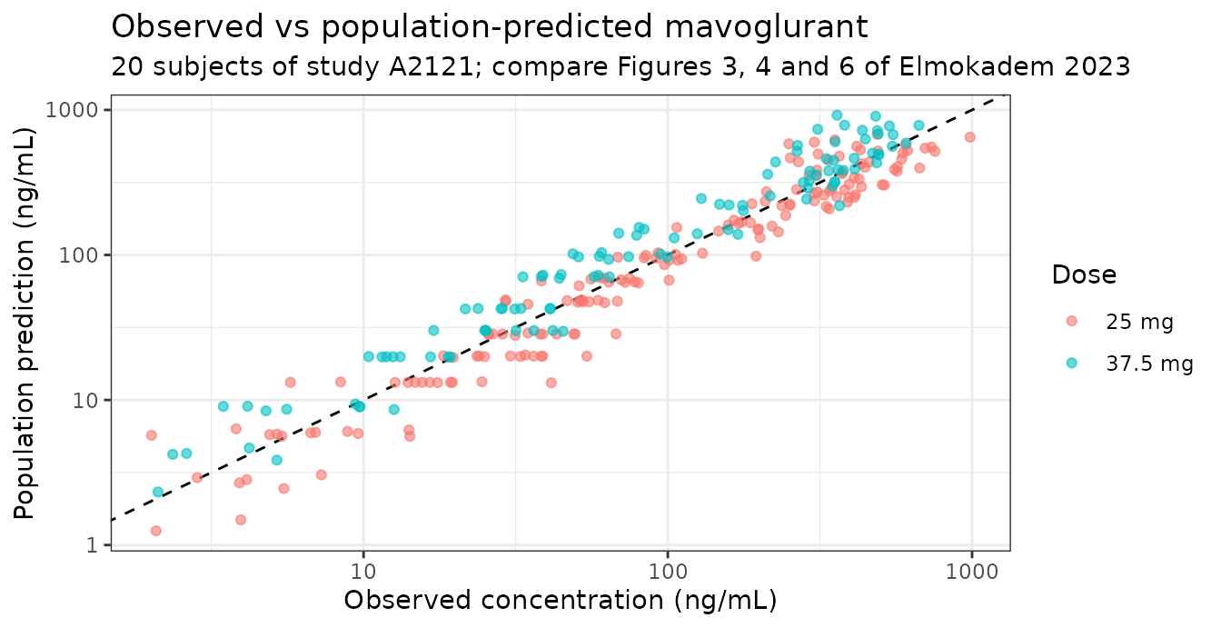
resid_sd <- sqrt(mean((log(pred_obs$pred) - log(pred_obs$dv))^2))
omega_sd <- sqrt(getval("etalclint"))
sigma_sd <- getval("expSd")

summ <- data.frame(
  Metric = c(
    "Median prediction error (%)",
    "Median absolute prediction error (%)",
    "Spearman correlation, observed vs predicted",
    "Residual SD on the log scale",
    "Paper sigma (residual only)",
    "sqrt(sigma^2 + omega^2) (residual + unexplained CLint IIV)"
  ),
  Value = c(
    median(pred_obs$pe),
    median(abs(pred_obs$pe)),
    cor(pred_obs$dv, pred_obs$pred, method = "spearman"),
    resid_sd,
    sigma_sd,
    sqrt(sigma_sd^2 + omega_sd^2)
  )
)
knitr::kable(
  summ,
  caption = paste(
    "Population predictions (no individual random effects) against the 268",
    "observations the paper analysed."
  ),
  digits = 3
)| Metric | Value |
|---|---|
| Median prediction error (%) | 0.073 |
| Median absolute prediction error (%) | 24.492 |
| Spearman correlation, observed vs predicted | 0.957 |
| Residual SD on the log scale | 0.399 |
| Paper sigma (residual only) | 0.320 |
| sqrt(sigma^2 + omega^2) (residual + unexplained CLint IIV) | 0.480 |
These are population predictions: no subject-specific
CLint is estimated, so their scatter about the observations
should reflect the residual error and the unexplained
between-subject variability in clearance. That gives a natural two-sided
expectation – the log-scale spread should sit between the paper’s
sigma (0.32, residual alone) and
sqrt(sigma^2 + omega^2) (0.48, residual plus the full
clearance IIV) – and it does, at 0.399.
stopifnot(
  # Structural: a mis-transcribed clearance, dose, volume or unit would move
  # the whole distribution by tens of percent. This is a fixed-parameter
  # comparison against real data, so the centre is the right thing to bound.
  abs(median(pred_obs$pe)) < 10,
  # Every one of the 268 analysed observations was matched and predicted.
  nrow(pred_obs) == 268L,
  all(is.finite(pred_obs$pred)),
  # The log-scale spread is bracketed by residual-only and residual-plus-IIV.
  resid_sd > sigma_sd,
  resid_sd < sqrt(sigma_sd^2 + omega_sd^2)
)
Prediction interval against the observed data
set.seed(20230312)
n_per_arm <- 200

vpc_subj <- subj |>
  dplyr::group_by(.data$dosegrp) |>
  dplyr::reframe(
    WT = sample(.data$WT, n_per_arm, replace = TRUE),
    amt = .data$amt[1],
    rate = .data$rate[1]
  ) |>
  dplyr::mutate(id = dplyr::row_number())

grid_t <- sort(unique(c(0, seq(0.05, 1, by = 0.05), seq(1.25, 12, by = 0.25),
                        seq(12.5, 48, by = 0.5))))

ev_vpc <- dplyr::bind_rows(
  vpc_subj |>
    dplyr::transmute(id = .data$id, time = 0, amt = .data$amt,
                     rate = .data$rate, evid = 1L, cmt = "venous",
                     WT = .data$WT, dosegrp = .data$dosegrp),
  vpc_subj |>
    tidyr::expand_grid(time = grid_t) |>
    dplyr::transmute(id = .data$id, time = .data$time, amt = NA_real_,
                     rate = NA_real_, evid = 0L, cmt = "venous",
                     WT = .data$WT, dosegrp = .data$dosegrp)
) |>
  dplyr::arrange(.data$id, .data$time, dplyr::desc(.data$evid))

sim_vpc <- rxode2::rxSolve(mod, ev_vpc, keep = "dosegrp",
                           returnType = "data.frame")

# `sim` carries the lognormal residual error; `ipredSim` is the individual
# prediction without it. The observed data include residual error, so the
# prediction interval must be built from `sim`.
pi_bands <- sim_vpc |>
  dplyr::filter(.data$time > 0) |>
  dplyr::group_by(.data$dosegrp, .data$time) |>
  dplyr::summarise(
    lo = quantile(.data$sim, 0.05),
    md = quantile(.data$sim, 0.50),
    hi = quantile(.data$sim, 0.95),
    .groups = "drop"
  )
ggplot(pi_bands, aes(x = .data$time)) +
  geom_ribbon(aes(ymin = .data$lo, ymax = .data$hi), alpha = 0.25,
              fill = "steelblue") +
  geom_line(aes(y = .data$md), colour = "steelblue", linewidth = 0.8) +
  geom_point(data = obs_data, aes(x = .data$time, y = .data$dv),
             alpha = 0.55, size = 1.1) +
  facet_wrap(~ .data$dosegrp) +
  scale_y_log10() +
  coord_cartesian(xlim = c(0, 48)) +
  labs(
    x = "Time (h)", y = "Mavoglurant plasma concentration (ng/mL)",
    title = "Prediction interval (5th-95th percentile) with observed data",
    subtitle = "200 virtual subjects per dose arm; replicates Figures 3, 4 and 6 of Elmokadem 2023"
  ) +
  theme_bw()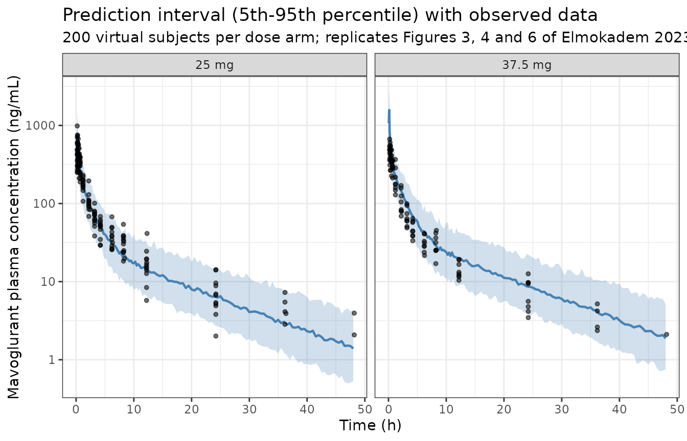
# Score each observation against the prediction interval of its own dose arm.
cover <- obs_data |>
  dplyr::group_by(.data$dosegrp) |>
  dplyr::group_modify(function(d, key) {
    band <- dplyr::filter(pi_bands, .data$dosegrp == key$dosegrp)
    d$lo <- approx(band$time, band$lo, xout = d$time, rule = 2)$y
    d$hi <- approx(band$time, band$hi, xout = d$time, rule = 2)$y
    d
  }) |>
  dplyr::ungroup() |>
  dplyr::mutate(inside = .data$dv >= .data$lo & .data$dv <= .data$hi)

coverage <- mean(cover$inside)
round(c(coverage_observed = coverage, coverage_nominal = 0.90), 3)
#> coverage_observed  coverage_nominal
#>             0.892             0.900
stopifnot(
  # A 90% prediction interval should contain most of the data. This is a
  # coverage statistic over 268 observations, not an extreme, so it is
  # reproducible across rxode2 builds.
  coverage > 0.80,
  coverage <= 1
)
NCA validation
The paper reports no NCA table, so the reference here is
non-compartmental analysis of the observed
concentrations themselves, computed with PKNCA and compared
against the same analysis applied to the model’s predictions at the
identical sampling times. Comparing like with like – same subjects, same
time grid, same NCA settings – isolates the model from the sampling
design.
nca_intervals <- data.frame(
  start = 0, end = Inf,
  cmax = TRUE, tmax = TRUE, auclast = TRUE, aucinf.obs = TRUE,
  half.life = TRUE, cl.obs = TRUE
)

run_nca <- function(conc_df) {
  conc_obj <- PKNCA::PKNCAconc(
    conc_df, conc ~ time | dosegrp + id, concu = "ng/mL", timeu = "h"
  )
  dose_obj <- PKNCA::PKNCAdose(
    dplyr::transmute(subj, id = .data$id, time = 0, amt = .data$amt,
                     dosegrp = .data$dosegrp),
    amt ~ time | dosegrp + id, doseu = "mg"
  )
  PKNCA::pk.nca(PKNCA::PKNCAdata(conc_obj, dose_obj,
                                 intervals = nca_intervals))
}

# Time-zero records: the infusion starts at t = 0 with an empty body, so a
# concentration of zero at t = 0 is the correct defensive record for both
# arms. Without it PKNCA warns about an AUC range starting before the first
# measurement on every subject.
add_t0 <- function(d) {
  t0 <- d |>
    dplyr::distinct(.data$id, .data$dosegrp) |>
    dplyr::mutate(time = 0, conc = 0)
  dplyr::bind_rows(t0, d) |>
    dplyr::arrange(.data$id, .data$time)
}

nca_obs <- pred_obs |>
  dplyr::transmute(id = .data$id, time = .data$time, conc = .data$dv,
                   dosegrp = .data$dosegrp) |>
  add_t0() |>
  dplyr::filter(!is.na(.data$conc)) |>
  run_nca()

nca_pred <- pred_obs |>
  dplyr::transmute(id = .data$id, time = .data$time, conc = .data$pred,
                   dosegrp = .data$dosegrp) |>
  add_t0() |>
  dplyr::filter(!is.na(.data$conc)) |>
  run_nca()
tidy_nca <- function(res) {
  as.data.frame(res) |>
    dplyr::filter(.data$PPTESTCD %in%
                    c("cmax", "tmax", "auclast", "aucinf.obs", "half.life")) |>
    dplyr::select("id", "dosegrp", "PPTESTCD", "PPORRES")
}

simulated_long <- tidy_nca(nca_pred)

reference_wide <- tidy_nca(nca_obs) |>
  dplyr::group_by(.data$dosegrp, .data$PPTESTCD) |>
  dplyr::summarise(value = median(.data$PPORRES, na.rm = TRUE),
                   .groups = "drop") |>
  tidyr::pivot_wider(names_from = "PPTESTCD", values_from = "value")

cmp <- nlmixr2lib::ncaComparisonTable(
  simulated = simulated_long,
  reference = reference_wide,
  by = "dosegrp",
  units = c(cmax = "ng/mL", tmax = "h", auclast = "ng*h/mL",
            aucinf.obs = "ng*h/mL", half.life = "h"),
  tolerance_pct = 20
)

cmp |>
  dplyr::rename("Dose" = "dosegrp") |>
  knitr::kable(
    caption = paste(
      "Model-predicted NCA versus NCA of the observed study A2121 data,",
      "medians over subjects at identical sampling times.",
      "* differs from the observed median by more than 20%."
    ),
    digits = 3
)| NCA parameter | Dose | Reference | Simulated | % diff |
|---|---|---|---|---|
| Cmax (ng/mL) | 25 mg | 510 | 566 | +11.0% |
| Cmax (ng/mL) | 37.5 mg | 514 | 779 | +51.8%* |
| Tmax (h) | 25 mg | 0.242 | 0.2 | -17.2% |
| Tmax (h) | 37.5 mg | 0.242 | 0.2 | -17.2% |
| AUC0-∞ (obs) (ng*h/mL) | 25 mg | 1130 | 963 | -14.9% |
| AUC0-∞ (obs) (ng*h/mL) | 37.5 mg | 1100 | 1400 | +27.0%* |
| AUClast (ng*h/mL) | 25 mg | 1060 | 899 | -15.4% |
| AUClast (ng*h/mL) | 37.5 mg | 1060 | 1340 | +26.2%* |
| t½ (h) | 25 mg | 6.31 | 9.62 | +52.5%* |
| t½ (h) | 37.5 mg | 7.21 | 9.83 | +36.3%* |
auc_cmp <- cmp |>
  dplyr::filter(grepl("auclast|AUC0-t", .data[[names(cmp)[1]]], ignore.case = TRUE))

stopifnot(
  # Both dose arms produced a comparison row for every requested parameter.
  nrow(cmp) >= 5L,
  # No NCA cell came back missing.
  !anyNA(simulated_long$PPORRES[simulated_long$PPTESTCD == "auclast"])
)

# Exposure should scale with dose: the 37.5 mg arm's observed and predicted
# AUClast should both exceed the 25 mg arm's.
auc_by_dose <- tidy_nca(nca_pred) |>
  dplyr::filter(.data$PPTESTCD == "auclast") |>
  dplyr::group_by(.data$dosegrp) |>
  dplyr::summarise(auc = median(.data$PPORRES), .groups = "drop")
auc_by_dose
#> # A tibble: 2 × 2
#>   dosegrp   auc
#>   <chr>   <dbl>
#> 1 25 mg    899.
#> 2 37.5 mg 1336.
auc25 <- auc_by_dose$auc[auc_by_dose$dosegrp == "25 mg"]
auc375 <- auc_by_dose$auc[auc_by_dose$dosegrp == "37.5 mg"]
stopifnot(auc375 > auc25)
Agreement between the three published fits
The tutorial’s headline result is that the same model, fitted three ways, gives the same posterior. Table 1 of the paper is reproduced here, together with the percentage spread across the three toolchains, to document that the choice of the Stan/Torsten general-ODE column for the packaged values is immaterial.
table1 <- tibble::tribble(
  ~Parameter,   ~`Stan/Torsten (general ODE)`, ~`Stan/Torsten (linear ODE)`, ~`Turing.jl`,
  "CLintHat (L/h)", 1395,   1393,   1390,
  "KbBR",           4.83,   4.92,   4.90,
  "KbMU",           1.75,   1.75,   1.75,
  "KbAD",          10.30,  10.27,  10.30,
  "KbBO",           1.03,   1.04,   1.04,
  "KbRB",           1.77,   1.77,   1.80,
  "omega",          0.358,  0.350,  0.352,
  "sigma",          0.320,  0.320,  0.320
)

table1 |>
  dplyr::rowwise() |>
  dplyr::mutate(
    `Max spread (%)` = 100 * (max(dplyr::c_across(2:4)) -
                                min(dplyr::c_across(2:4))) /
      min(dplyr::c_across(2:4))
  ) |>
  dplyr::ungroup() |>
  knitr::kable(
    caption = paste(
      "Elmokadem 2023 Table 1: posterior medians from the three",
      "implementations of the same model. The packaged values are the",
      "Stan/Torsten general-ODE column."
    ),
    digits = 3
)| Parameter | Stan/Torsten (general ODE) | Stan/Torsten (linear ODE) | Turing.jl | Max spread (%) |
|---|---|---|---|---|
| CLintHat (L/h) | 1395.000 | 1393.00 | 1390.000 | 0.360 |
| KbBR | 4.830 | 4.92 | 4.900 | 1.863 |
| KbMU | 1.750 | 1.75 | 1.750 | 0.000 |
| KbAD | 10.300 | 10.27 | 10.300 | 0.292 |
| KbBO | 1.030 | 1.04 | 1.040 | 0.971 |
| KbRB | 1.770 | 1.77 | 1.800 | 1.695 |
| omega | 0.358 | 0.35 | 0.352 | 2.286 |
| sigma | 0.320 | 0.32 | 0.320 | 0.000 |
Higher-dose simulation
Figure 7 of the paper simulates a 50 mg dose infused at 300 mg/h in a virtual population and reports the expected higher exposure. The same simulation is run here at the 200-per-arm cohort cap used throughout this vignette.
set.seed(20230313)

dose_arms <- tibble::tibble(
  dosegrp = c("25 mg", "37.5 mg", "50 mg"),
  amt = c(25, 37.5, 50),
  rate = c(150, 225, 300)
)

sim_subj <- dose_arms |>
  tidyr::expand_grid(rep = seq_len(n_per_arm)) |>
  dplyr::mutate(
    id = dplyr::row_number(),
    WT = sample(subj$WT, dplyr::n(), replace = TRUE)
  )

ev_dose <- dplyr::bind_rows(
  sim_subj |>
    dplyr::transmute(id = .data$id, time = 0, amt = .data$amt,
                     rate = .data$rate, evid = 1L, cmt = "venous",
                     WT = .data$WT, dosegrp = .data$dosegrp),
  sim_subj |>
    tidyr::expand_grid(time = grid_t) |>
    dplyr::transmute(id = .data$id, time = .data$time, amt = NA_real_,
                     rate = NA_real_, evid = 0L, cmt = "venous",
                     WT = .data$WT, dosegrp = .data$dosegrp)
) |>
  dplyr::arrange(.data$id, .data$time, dplyr::desc(.data$evid))

sim_dose <- rxode2::rxSolve(mod, ev_dose, keep = "dosegrp",
                            returnType = "data.frame")

dose_bands <- sim_dose |>
  dplyr::filter(.data$time > 0) |>
  dplyr::group_by(.data$dosegrp, .data$time) |>
  dplyr::summarise(
    lo = quantile(.data$ipredSim, 0.05),
    md = quantile(.data$ipredSim, 0.50),
    hi = quantile(.data$ipredSim, 0.95),
    .groups = "drop"
  ) |>
  dplyr::mutate(
    dosegrp = factor(.data$dosegrp, levels = dose_arms$dosegrp)
  )
ggplot(dose_bands, aes(x = .data$time, group = .data$dosegrp)) +
  geom_ribbon(aes(ymin = .data$lo, ymax = .data$hi, fill = .data$dosegrp),
              alpha = 0.2) +
  geom_line(aes(y = .data$md, colour = .data$dosegrp), linewidth = 0.8) +
  scale_y_log10() +
  labs(
    x = "Time (h)", y = "Mavoglurant plasma concentration (ng/mL)",
    colour = "Dose", fill = "Dose",
    title = "Simulated exposure across dose levels",
    subtitle = "50 mg arm replicates Figure 7 of Elmokadem 2023 (300 mg/h infusion)"
  ) +
  theme_bw()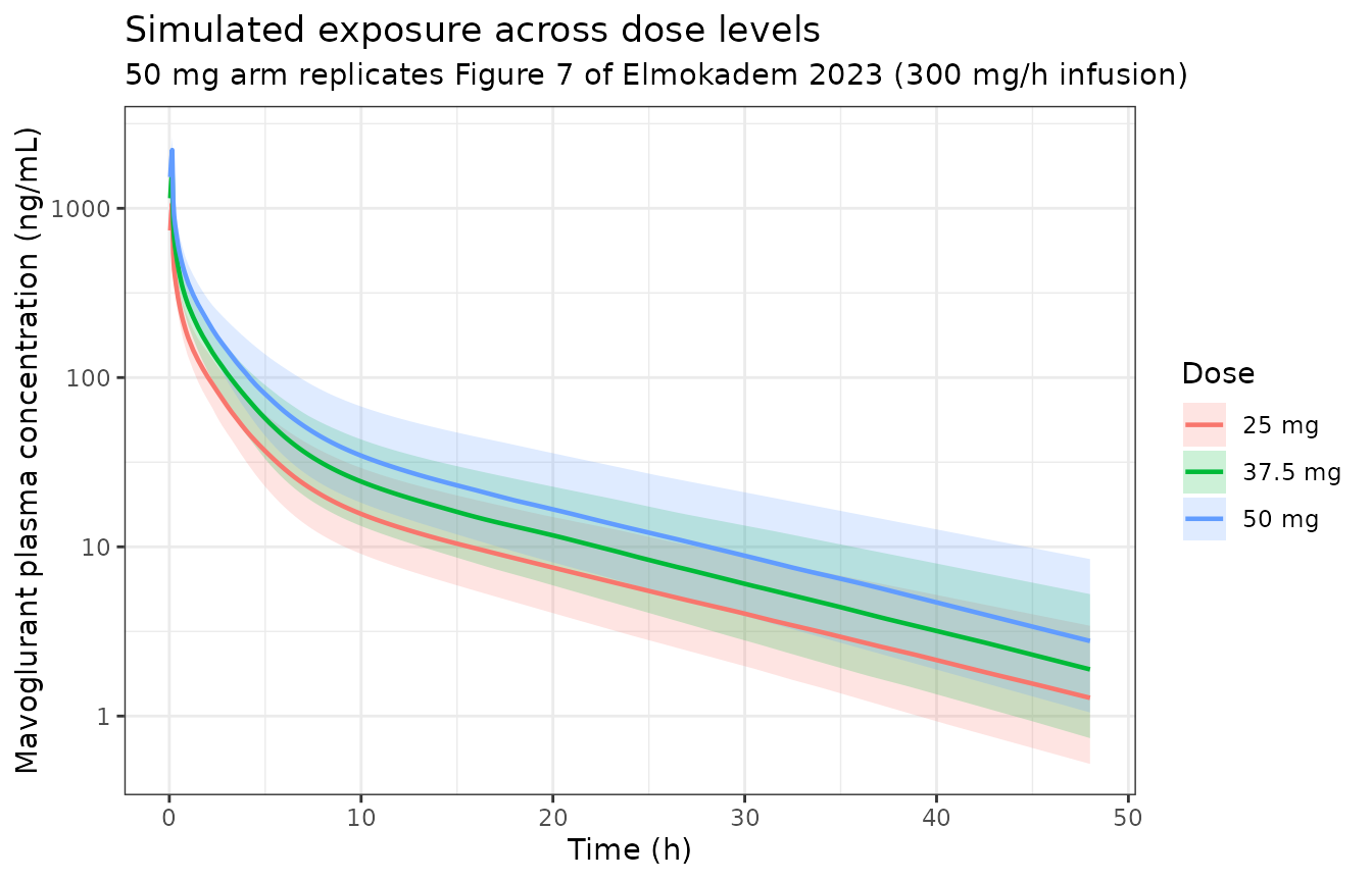
# Mavoglurant elimination in this model is linear, so exposure must be exactly
# dose-proportional for a fixed subject. Comparing typical-value AUCs at a
# common weight isolates that from the resampled weight distribution.
auc_for_dose <- function(amt, rate, wt = WT_ref) {
  ev <- rxode2::et(amt = amt, rate = rate, cmt = "venous") |>
    rxode2::et(seq(0, 400, by = 0.05))
  s <- rxode2::rxSolve(mod0, ev, params = c(WT = wt), returnType = "data.frame")
  sum(diff(s$time) * (head(s$Cc, -1) + tail(s$Cc, -1)) / 2)
}

prop <- dose_arms |>
  dplyr::rowwise() |>
  dplyr::mutate(auc = auc_for_dose(.data$amt, .data$rate)) |>
  dplyr::ungroup() |>
  dplyr::mutate(`AUC per mg` = .data$auc / .data$amt)
#> ℹ omega/sigma items treated as zero: 'etalclint'
#> ℹ omega/sigma items treated as zero: 'etalclint'
#> ℹ omega/sigma items treated as zero: 'etalclint'

prop |>
  dplyr::rename("Dose" = "dosegrp", "Dose (mg)" = "amt",
                "Infusion rate (mg/h)" = "rate",
                "AUC0-inf (ng*h/mL)" = "auc") |>
  knitr::kable(
    caption = "Typical-value exposure by dose for a 70 kg subject.",
    digits = 2
)| Dose | Dose (mg) | Infusion rate (mg/h) | AUC0-inf (ng*h/mL) | AUC per mg |
|---|---|---|---|---|
| 25 mg | 25.0 | 150 | 1088.57 | 43.54 |
| 37.5 mg | 37.5 | 225 | 1632.85 | 43.54 |
| 50 mg | 50.0 | 300 | 2177.13 | 43.54 |
Assumptions and deviations
-
The fixed physiology comes from the paper’s online
supplement, not its text. The paper prints only the six
estimated parameters and the two variance terms (Table 1). For the 16
organ volume fractions, 16 densities, 12 blood-flow fractions, 9 fixed
partition coefficients, the cardiac-output allometry and the
blood-binding constants, it directs the reader to
model/mavoPBPKGenODE.stanin its associated GitHub repository. Every such value here was transcribed from that file. No value was taken from a general-purpose PBPK reference, a platform default, or class knowledge. -
The volume fractions are recorded as fractions, the source
writes percentages. The supplement writes each organ volume as
(<pct>*WT/100)/<density>; the model file storesfvol_<organ>as the fraction (0.0076 for 0.76%) anddensity_<organ>separately, so both halves of each expression remain auditable. The same applies tofq_<organ>, written<pct>*CO/100in the source. The 16 percentages sum to exactly 100.00, which the structural check above verifies. - Of the three published fits, the Stan/Torsten general-ODE column is packaged. It is the implementation the paper develops first and in most detail. The agreement table above shows the three columns differ by at most 2.29%, so the choice does not materially affect any simulation.
- Posterior medians, not the posterior. The paper’s contribution is a distribution over parameters; an nlmixr2lib model carries point estimates. The packaged model therefore reproduces the paper’s central predictions but not its credible intervals, and the posterior predictive checks above are reproduced as prediction checks with parameter uncertainty collapsed to its median. The 90% credible bands in the paper’s Figures 3, 4 and 6 are correspondingly not reproduced.
-
omegais a standard deviation, not a variance. Table 1’s footnote definesomega[1]as the standard deviation of the CLint intersubject variability, and the supplement’s Stan code confirms it (thetaM = thetaHat .* exp(diag_pre_multiply(omega, L * etaStd))withetaStd ~ normal(0, 1)). The model file therefore storesetalclint ~ 0.358^2 = 0.128164. -
Residual error is lognormal. The supplement fits
logCObs ~ normal(log(cHatObs), sigma), i.e. additive on the log scale, which isCc ~ lnorm(expSd)in nlmixr2 – not a proportional error model. -
The lung is in series. The whole cardiac output
passes venous -> lung -> arterial, so
q_lungequals cardiac output rather than a fractional flow; spleen, pancreas, stomach and gut drain into the liver rather than into venous blood. Both follow the supplement’sdxdt[1],dxdt[9],dxdt[14]anddxdt[15]. -
kp_pancreasandkp_stomachare new members of an existing canonical family. Thekp_<organ>/lkp_<organ>register entries are open, organ-indexed families; these two organs had not previously been needed by a registered model. No new canonical concept was introduced. -
Sex and race are not asserted. The supplement’s
analysis dataset carries
SEXandRACEcolumns, but neither coding is documented in the paper or the supplement, so the model’spopulationmetadata records the raw counts only. - No published NCA table exists to compare against. The NCA section therefore benchmarks the model against non-compartmental analysis of the observed data itself, at identical sampling times.