Benzylpenicillin (Yoo 2025)

Model and source

• Citation: Yoo O, Salman S, Hla TK, Osowicki J, Page-Sharp M, Marsh JA, Barr R, Azzopardi K, Morici M, Batty KT, Enkel SL, Kado J, Hatchuel L, Fulurija A, McCarthy JS, Snelling T, Steer AC, Carapetis J, Manning L. Population pharmacokinetics of penicillin G: insights into increased clearance at low concentrations to guide development of improved long-acting formulations for syphilis and prevention of rheumatic fever. Antimicrob Agents Chemother. 2025;69(7):e00269-25. doi:10.1128/aac.00269-25
• Description: Two-compartment population PK model for intravenous benzylpenicillin (penicillin G) in healthy adult volunteers of the CHIPS human-challenge trial (Yoo 2025), fitted jointly to a 600 mg IV bolus and to low-dose continuous IV infusions targeting 3-20 ng/mL; clearance is proportional to cystatin-C-based eGFR in absolute mL/min, the central volume is 1.96-fold larger during continuous infusion, and clearance rises by an additive 12.1 L/h during infusion at the 3 ng/mL target
• Article: https://doi.org/10.1128/aac.00269-25 (open access, PMC12217478)

Yoo 2025 analysed the pharmacokinetic run-in and the infusion phase of the CHIPS controlled human pharyngitis challenge trial. Every participant first received a single 600 mg intravenous benzylpenicillin dose over 3 minutes; 7-35 days later, participants were randomized to a loading dose plus a continuous infusion individualized to a target steady-state concentration (Css) of 3, 6, 9, 12 or 20 ng/mL, the infusion rate being the target Css multiplied by the participant’s clearance from the bolus (the paper’s equation 1, Infusion rate = Clearance x Css). Both phases were fitted jointly with a two-compartment model in NONMEM 7.5.1 (FOCE-I). The final model (Table 4) has three non-standard features:

• clearance is proportional to the cystatin-C-based CKD-EPI 2012 eGFR in absolute mL/min (eGFR in mL/min/1.73 m^2 multiplied by the Mosteller body-surface area over 1.73), with no body-weight effect on CL;
• the central volume is 1.96-fold larger during continuous infusion than during the bolus (REGIMEN_CONTINF);
• clearance rises by an additive 12.1 L/h, with 42.9% inter-individual variability, on the infusion records of the 3 ng/mL target arm only (DOSE_LOW). This is the paper’s headline finding: at that target, the measured concentrations fell below the concentration the bolus clearance predicted.

Population

Seventy-two healthy adult volunteers (42% female, median age 25 years, range 18-38; median weight 69 kg, range 50-107; median BSA 1.79 m^2; median serum creatinine 70 umol/L and cystatin C 0.59 mg/L; Table 1) contributed 504 bolus samples (0.25, 0.5, 1, 2, 3, 4 and 6 h post-dose). Forty-seven of them received a continuous infusion and contributed 389 samples drawn every 12 h; Table 2 lists 10, 9, 10, 9 and 9 participants in the 3, 6, 9, 12 and 20 ng/mL arms. The trial ran in Perth, Australia, between August 2022 and July 2023. Race and ethnicity are not reported.

The same information is available programmatically via readModelDb("Yoo_2025_benzylpenicillin")()$population.

Source trace

Equation / parameter	Value	Source location
lcl (CL at eGFRcys = 60 mL/min)	log(13.3) L/h	Table 4, CL = theta x eGFRcys/60, theta = 13.3 (RSE 2%)
lvc (Vc, bolus phase, 70 kg)	log(14.6) L	Table 4
lq (Q, 70 kg)	log(5.34) L/h	Table 4
lvp (Vp, 70 kg)	log(5.77) L	Table 4
e_wt_vc, e_wt_vp	1 (fixed)	Methods, ‘Population pharmacokinetic analysis’ (allometry applied a priori)
e_wt_q	0.75 (fixed)	Methods, ‘Population pharmacokinetic analysis’
e_regimen_continf_vc	1.96	Table 4 Ratio,Vc; Vc,Linf = Vc x Ratio,Vc
e_dose_low_cl	12.1 L/h	Table 4 Difference,CL,Css3; CL_Css3 = CL + Difference
etalcl	0.144^2	Table 4 IIV CL 14.4% (shrinkage 6%)
etalvc	0.169^2	Table 4 IIV VC 16.9% (shrinkage 22%)
etalvp	0.137^2	Table 4 IIV Vp 13.7% (shrinkage 15%)
etae_dose_low_cl	0.429^2	Table 4 IIV Difference,CL,Css3 42.9% (shrinkage 69%)
propSd	0.165	Table 4 ‘Proportional error (%)’ 16.5% (shrinkage 10%)
CRCL = eGFRcys x BSA / 1.73	n/a	Methods, ‘Benzylpenicillin clearance predictor’
BSA = sqrt(height x weight / 3600)	n/a	Methods, equation 2 (Mosteller)
Two-compartment ODEs, first-order elimination	n/a	Results and Methods, ‘Population pharmacokinetic analysis’

Virtual cohort

The observed data are not public. The cohort below draws body weight, height, age, sex and cystatin C to match Table 1, then computes the Mosteller BSA, the CKD-EPI 2012 cystatin C eGFR and its absolute-mL/min form, which is the model’s CRCL column. One hundred subjects are assigned to each of the five target arms.

The random effects are drawn here in R rather than by rxSolve(), for two reasons. The trial set each participant’s infusion rate from that participant’s own bolus clearance, so the rate has to be known before the solve. And drawing the etas with set.seed() makes every clearance-based check below identical on every machine; only the residual error is left to rxode2’s random-number stream.

set.seed(20250520)

n_per_arm <- 100
arms <- c(3, 6, 9, 12, 20)
n_sub <- n_per_arm * length(arms)

# Log-normal draw with reject-and-redraw inside the observed range; the
# range is a definition of the cohort, so values are never clamped.
rlnorm_range <- function(n, median, cv, lo, hi) {
  x <- rlnorm(n, log(median), sqrt(log(cv^2 + 1)))
  bad <- x < lo | x > hi
  while (any(bad)) {
    x[bad] <- rlnorm(sum(bad), log(median), sqrt(log(cv^2 + 1)))
    bad <- x < lo | x > hi
  }
  x
}

# CKD-EPI cystatin C age-sex equation (Inker 2012), mL/min/1.73 m^2.
egfr_cys_2012 <- function(scys, age, sexf) {
  133 * pmin(scys / 0.8, 1)^-0.499 * pmax(scys / 0.8, 1)^-1.328 *
    0.996^age * ifelse(sexf == 1, 0.932, 1)
}

cohort <- tibble(
  id = seq_len(n_sub),
  arm = rep(arms, each = n_per_arm),
  WT = rlnorm_range(n_sub, 69, 0.18, 50, 107),
  HT = rlnorm_range(n_sub, 170, 0.06, 144, 192),
  AGE = rlnorm_range(n_sub, 25, 0.19, 18, 38),
  SEXF = rbinom(n_sub, 1, 0.42),
  CYSC = rlnorm_range(n_sub, 0.59, 0.168, 0.39, 0.87)
) |>
  mutate(
    BSA = sqrt(HT * WT / 3600),
    EGFR_CYS = egfr_cys_2012(CYSC, AGE, SEXF),
    CRCL = EGFR_CYS * BSA / 1.73
  )

# Individual random effects on the SD scale of Table 4 (see Assumptions).
omega_sd <- c(etalcl = 0.144, etalvc = 0.169, etalvp = 0.137, etae_dose_low_cl = 0.429)
etas <- as_tibble(lapply(omega_sd, function(s) rnorm(n_sub, 0, s))) |>
  mutate(id = cohort$id, .before = 1)

cohort <- cohort |>
  left_join(etas, by = "id") |>
  mutate(
    # Bolus-phase individual clearance (L/h) and the trial's infusion rate,
    # equation 1: rate = CL x Css. Css in ng/mL = ug/L; rate in mg/h.
    cl_bolus = 13.3 * exp(etalcl) * CRCL / 60,
    rate_mg_h = cl_bolus * arm / 1000
  )

cohort |>
  summarise(
    `Weight (kg)` = median(WT), `Height (cm)` = median(HT),
    `BSA (m^2)` = median(BSA), `Cystatin C (mg/L)` = median(CYSC),
    `eGFRcys (mL/min/1.73 m^2)` = median(EGFR_CYS),
    `CRCL (mL/min)` = median(CRCL)
  ) |>
  knitr::kable(digits = 2, caption = "Virtual-cohort medians.")

Virtual-cohort medians.

Weight (kg)	Height (cm)	BSA (m^2)	Cystatin C (mg/L)	eGFRcys (mL/min/1.73 m^2)	CRCL (mL/min)
68.38	169.42	1.8	0.6	134.66	140.34

The cohort’s median BSA lands within 0.03 m^2 of Table 1, and its median infusion rate per arm can be set beside Table 2:

table2_rate <- tibble(
  arm = arms,
  table2_median_rate = c(80.3, 220.4, 347.1, 367.5, 592.4)
)
rate_cmp <- cohort |>
  group_by(arm) |>
  summarise(sim_median_rate = median(rate_mg_h) * 1000, .groups = "drop") |>
  left_join(table2_rate, by = "arm") |>
  mutate(pct_diff = 100 * (sim_median_rate / table2_median_rate - 1))
rate_cmp |>
  rename(
    "Target Css (ng/mL)" = arm,
    "Simulated median rate (ug/h)" = sim_median_rate,
    "Table 2 median rate (ug/h)" = table2_median_rate,
    "% difference" = pct_diff
  ) |>
  knitr::kable(digits = 1, caption = "Infusion rate = bolus clearance x target Css, by arm.")

Infusion rate = bolus clearance x target Css, by arm.

Target Css (ng/mL)	Simulated median rate (ug/h)	Table 2 median rate (ug/h)	% difference
3	96.2	80.3	19.8
6	194.0	220.4	-12.0
9	279.5	347.1	-19.5
12	366.0	367.5	-0.4
20	613.3	592.4	3.5

stopifnot(
  abs(median(cohort$BSA) - 1.79) < 0.03,
  # Rates scale with the target by construction; this pins the clearance
  # magnitude. Table 2's arms differ from each other by up to 44% in
  # rate / Css, so the band is the across-arm spread, not a tight match.
  all(abs(rate_cmp$pct_diff) < 30)
)

Simulation

Each subject receives the 600 mg bolus over 3 minutes at time 0 and starts a 96-hour infusion at day 14 (336 h), long after the bolus has cleared. The two indicator covariates are 0 during the bolus phase; during the infusion REGIMEN_CONTINF = 1 for every arm and DOSE_LOW = 1 for the 3 ng/mL arm. Both are written on every row, including the observation rows.

t_inf <- 336
dur_inf <- 96
bolus_times <- c(0, 0.05, 0.1, 0.15, 0.25, 0.5, 1, 2, 3, 4, 6, 8, 10, 12)
paper_bolus_times <- c(0.25, 0.5, 1, 2, 3, 4, 6)
inf_times <- t_inf + seq(12, dur_inf, by = 12)

dose_rows <- bind_rows(
  cohort |> transmute(id, time = 0, evid = 1L, amt = 600, rate = 600 / 0.05),
  cohort |> transmute(id, time = t_inf, evid = 1L, amt = rate_mg_h * dur_inf, rate = rate_mg_h)
)
obs_rows <- tidyr::expand_grid(id = cohort$id, time = c(bolus_times, inf_times)) |>
  mutate(evid = 0L, amt = 0, rate = 0)

events <- bind_rows(dose_rows, obs_rows) |>
  left_join(cohort |> select(id, arm, WT, CRCL), by = "id") |>
  mutate(
    cmt = "central",
    phase = ifelse(time >= t_inf, "infusion", "bolus"),
    REGIMEN_CONTINF = as.integer(time >= t_inf),
    DOSE_LOW = as.integer(time >= t_inf & arm == 3)
  ) |>
  arrange(id, time, desc(evid)) |>
  as.data.frame()

stopifnot(!anyDuplicated(events[, c("id", "time", "evid")]))

mod <- readModelDb("Yoo_2025_benzylpenicillin")
# The fixed effects come from ini(); the per-subject etas drawn above are
# supplied through `params`, so the model's omega is zeroed and only the
# proportional residual error is simulated by rxode2.
mod_fixed_eta <- rxode2::zeroRe(mod, which = "omega")
#> ℹ parameter labels from comments will be replaced by 'label()'
eta_params <- cohort |> select(id, all_of(names(omega_sd))) |> as.data.frame()

sim <- suppressWarnings(rxode2::rxSolve(
  mod_fixed_eta, events = events, params = eta_params,
  keep = c("arm", "phase"), returnType = "data.frame"
))

Replicate published figures

Figure 4A: bolus phase

sim |>
  filter(phase == "bolus", time %in% paper_bolus_times) |>
  group_by(time) |>
  summarise(
    Q05 = quantile(sim, 0.05), Q50 = quantile(sim, 0.50), Q95 = quantile(sim, 0.95),
    .groups = "drop"
  ) |>
  ggplot(aes(time, Q50)) +
  geom_ribbon(aes(ymin = Q05, ymax = Q95), alpha = 0.25) +
  geom_line() +
  geom_point() +
  scale_y_log10() +
  labs(
    x = "Time after the 600 mg bolus (h)", y = "Benzylpenicillin (mg/L)",
    title = "Bolus phase: simulated 5th, 50th and 95th percentiles",
    caption = "Replicates Figure 4A of Yoo 2025."
  )

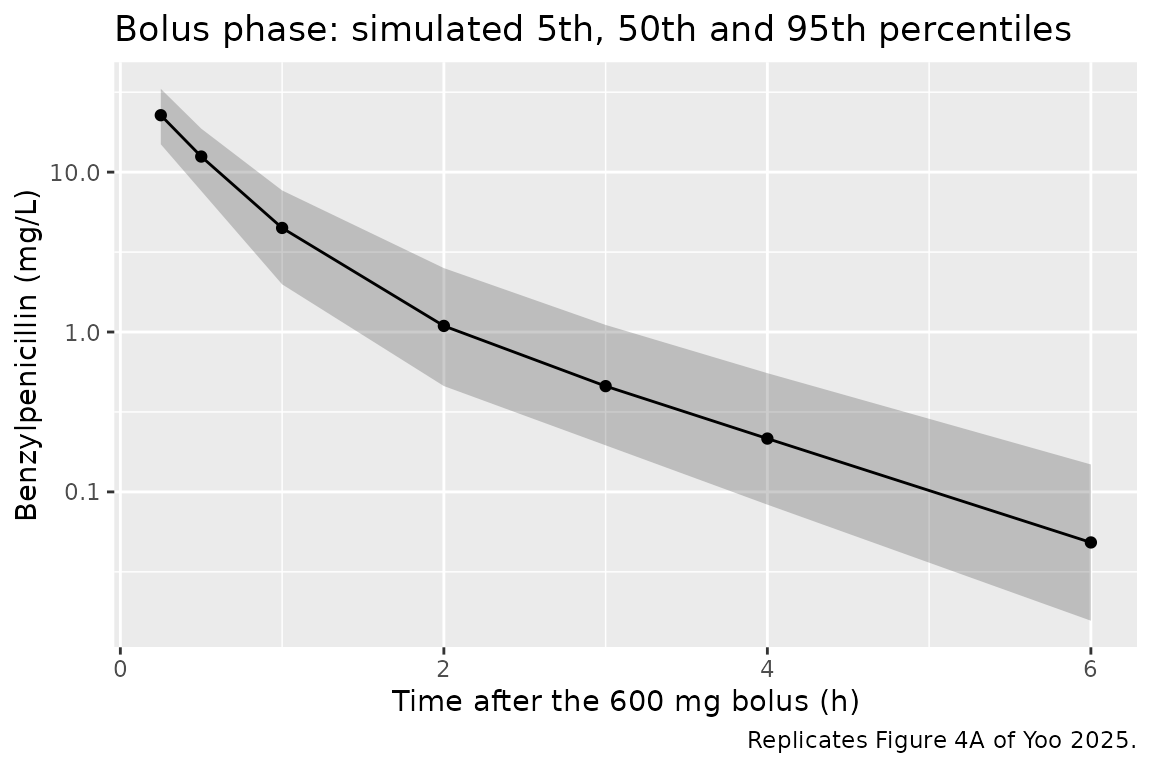
Figure 4B-F: continuous infusion by target

sim |>
  filter(phase == "infusion") |>
  mutate(time_inf = time - t_inf, conc_ng = sim * 1000) |>
  group_by(arm, time_inf) |>
  summarise(
    Q05 = quantile(conc_ng, 0.05), Q50 = quantile(conc_ng, 0.50), Q95 = quantile(conc_ng, 0.95),
    .groups = "drop"
  ) |>
  ggplot(aes(time_inf, Q50)) +
  geom_ribbon(aes(ymin = Q05, ymax = Q95), alpha = 0.25) +
  geom_line() +
  geom_hline(aes(yintercept = arm), linetype = "dashed", colour = "firebrick") +
  facet_wrap(~ paste("Target", arm, "ng/mL"), scales = "free_y") +
  labs(
    x = "Time after start of infusion (h)", y = "Benzylpenicillin (ng/mL)",
    title = "Infusion phase: simulated percentiles (dashed line = target Css)",
    caption = "Replicates Figure 4B-F of Yoo 2025 (infusion portion)."
  )

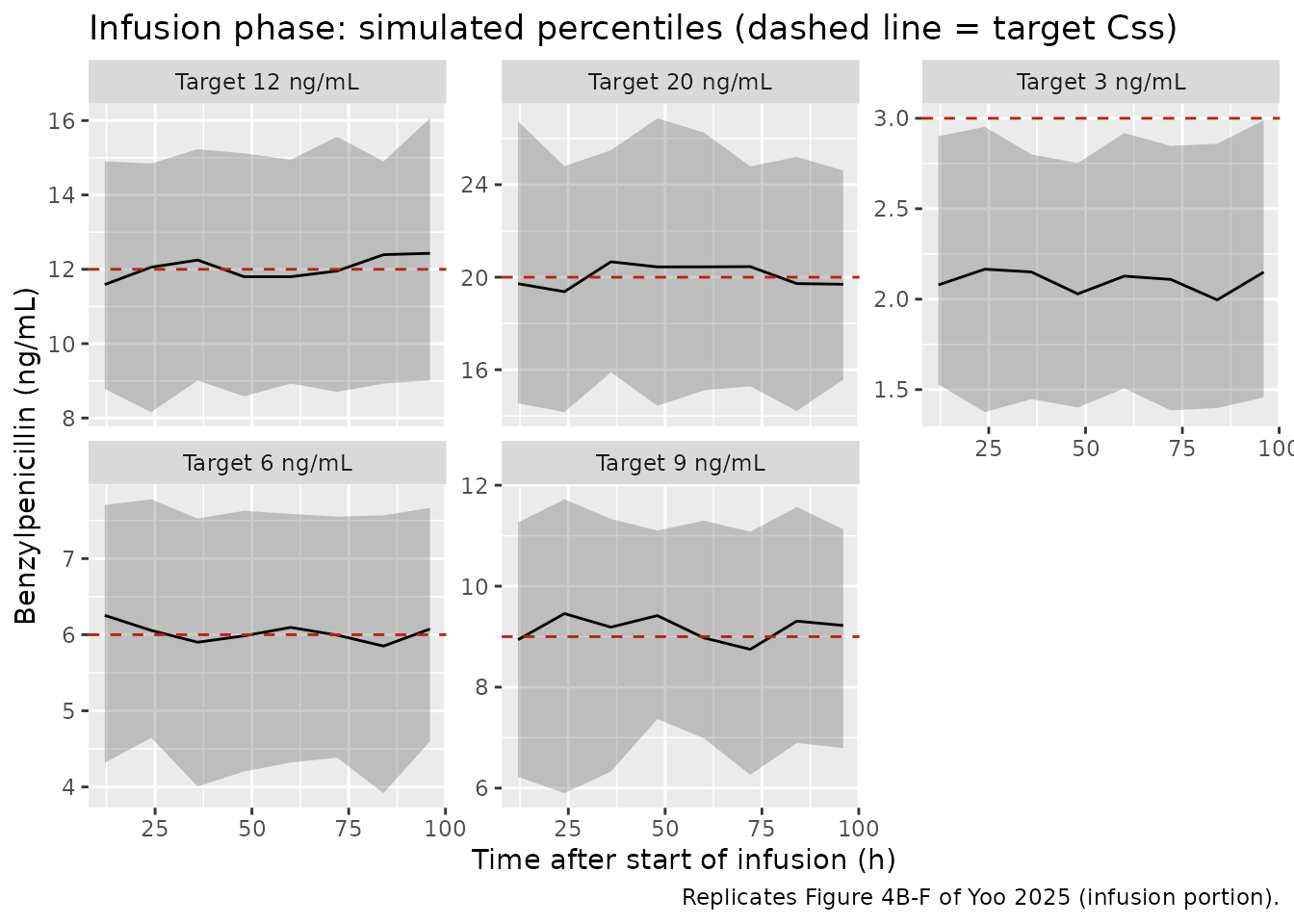
The 3 ng/mL arm sits below its target while the other four sit on theirs: the rate was set from the bolus clearance, and only that arm’s infusion clearance is higher.

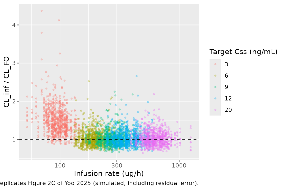
Figures 1 and 2: infusion clearance relative to bolus clearance

The paper computes an observed infusion clearance as rate / measured Css (equation 1) and normalizes it by the bolus clearance.

cl_ratio <- sim |>
  filter(phase == "infusion") |>
  left_join(cohort |> select(id, cl_bolus, rate_mg_h), by = "id") |>
  mutate(cl_inf_obs = rate_mg_h / sim, ratio = cl_inf_obs / cl_bolus)

ggplot(cl_ratio, aes(rate_mg_h * 1000, ratio, colour = factor(arm))) +
  geom_point(alpha = 0.3, size = 0.8) +
  geom_hline(yintercept = 1, linetype = "dashed") +
  scale_x_log10() +
  labs(
    x = "Infusion rate (ug/h)", y = "CL_inf / CL_FO",
    colour = "Target Css (ng/mL)",
    caption = "Replicates Figure 2C of Yoo 2025 (simulated, including residual error)."
  )

# Structural ratio without residual error: CL_inf / CL_bolus from the
# individual parameters. Arms 6-20 are 1 by construction; the 3 ng/mL arm
# is 1 + 12.1 * exp(eta) / CL_bolus.
struct_ratio <- sim |>
  filter(phase == "infusion", time == t_inf + dur_inf) |>
  left_join(cohort |> select(id, cl_bolus), by = "id") |>
  mutate(ratio = cl / cl_bolus) |>
  group_by(arm) |>
  summarise(
    median_ratio = median(ratio), p05 = quantile(ratio, 0.05), p95 = quantile(ratio, 0.95),
    .groups = "drop"
  )
knitr::kable(struct_ratio, digits = 2, caption = "Infusion-phase CL relative to bolus CL, by arm.")

Infusion-phase CL relative to bolus CL, by arm.

arm	median_ratio	p05	p95
3	1.4	1.17	1.79
6	1.0	1.00	1.00
9	1.0	1.00	1.00
12	1.0	1.00	1.00
20	1.0	1.00	1.00

ratio_3 <- struct_ratio$median_ratio[struct_ratio$arm == 3]
stopifnot(
  # The etas are drawn in R, so these are the same on every machine.
  abs(struct_ratio$median_ratio[struct_ratio$arm != 3] - 1) < 1e-8,
  # 12.1 L/h on a median bolus CL of about 31 L/h.
  ratio_3 > 1.25, ratio_3 < 1.55,
  # 42.9% IIV on the step: 12.1 * exp(1.645 * 0.429) = 24.4 L/h at the 95th
  # percentile of the step alone.
  struct_ratio$p95[struct_ratio$arm == 3] > 1.6,
  struct_ratio$p95[struct_ratio$arm == 3] < 2.1
)
obs_ratio_3 <- cl_ratio$ratio[cl_ratio$arm == 3]

The median 3 ng/mL subject clears benzylpenicillin about 40% faster during the infusion than after the bolus, and the structural 95th percentile is 1.79. Residual error spreads the ratio computed from simulated observations further: 7.5% of the 3 ng/mL samples exceed 2, the region Figures 1 and 2D of the paper show for that arm.

Analytical checks

Two identities that use the same drawn parameters on both sides, so they must hold to numerical precision.

# Steady state of a constant-rate infusion: Css = rate / CL.
ss <- sim |>
  filter(phase == "infusion", time == t_inf + dur_inf) |>
  left_join(cohort |> select(id, rate_mg_h), by = "id") |>
  mutate(rel_err = Cc / (rate_mg_h / cl) - 1)

# Bolus mass balance on a dense typical-value solve: CL * AUC(0-inf) = dose.
typ <- tibble(WT = 70, CRCL = 140)
ev_typ <- rxode2::et(amt = 600, rate = 600 / 0.05, cmt = "central") |>
  rxode2::et(c(seq(0, 1, by = 0.005), seq(1.01, 48, by = 0.01)))
sim_typ <- rxode2::rxSolve(
  rxode2::zeroRe(mod), ev_typ,
  params = c(CRCL = 140, WT = 70, REGIMEN_CONTINF = 0, DOSE_LOW = 0),
  returnType = "data.frame", atol = 1e-12, rtol = 1e-10
)
#> ℹ parameter labels from comments will be replaced by 'label()'
#> ℹ omega/sigma items treated as zero: 'etalcl', 'etalvc', 'etalvp', 'etae_dose_low_cl'
auc_typ <- sum(diff(sim_typ$time) * (head(sim_typ$Cc, -1) + tail(sim_typ$Cc, -1)) / 2)
cl_typ <- 13.3 * 140 / 60

c(
  max_ss_rel_err = max(abs(ss$rel_err)),
  cl_times_auc_over_dose = cl_typ * auc_typ / 600
)
#>         max_ss_rel_err cl_times_auc_over_dose 
#>           8.724191e-07           1.000003e+00
stopifnot(
  max(abs(ss$rel_err)) < 1e-4,
  abs(cl_typ * auc_typ / 600 - 1) < 1e-3
)

PKNCA validation

NCA of the bolus phase, per randomized arm. The grid adds 0.05, 0.1, 0.15, 8, 10 and 12 h to the paper’s sampling times so that AUC(0-inf) is not dominated by trapezoidal error on the 3-minute peak.

sim_nca <- sim |>
  filter(phase == "bolus", !is.na(Cc)) |>
  mutate(treatment = paste(arm, "ng/mL")) |>
  select(id, time, Cc, treatment)

sim_nca <- bind_rows(
  sim_nca,
  sim_nca |> distinct(id, treatment) |> mutate(time = 0, Cc = 0)
) |>
  distinct(id, treatment, time, .keep_all = TRUE) |>
  arrange(id, treatment, time)

dose_df <- events |>
  filter(evid == 1, time == 0) |>
  mutate(treatment = paste(arm, "ng/mL"), duration = 0.05) |>
  select(id, time, amt, duration, treatment)

conc_obj <- PKNCA::PKNCAconc(sim_nca, Cc ~ time | treatment + id)
dose_obj <- PKNCA::PKNCAdose(dose_df, amt ~ time | treatment + id,
                             route = "intravascular", duration = "duration")
intervals <- data.frame(
  start = 0, end = Inf,
  cmax = TRUE, tmax = TRUE, aucinf.obs = TRUE, half.life = TRUE, cl.obs = TRUE
)
nca_res <- PKNCA::pk.nca(PKNCA::PKNCAdata(conc_obj, dose_obj, intervals = intervals))
summary(nca_res)
#>  start end treatment   N        cmax                    tmax     half.life
#>      0 Inf  12 ng/mL 100 39.3 [24.3] 0.0500 [0.0500, 0.0500] 0.969 [0.136]
#>      0 Inf  20 ng/mL 100 38.6 [20.4] 0.0500 [0.0500, 0.0500] 0.980 [0.131]
#>      0 Inf   3 ng/mL 100 39.7 [20.1] 0.0500 [0.0500, 0.0500] 0.950 [0.130]
#>      0 Inf   6 ng/mL 100 37.8 [22.6] 0.0500 [0.0500, 0.0500] 0.964 [0.162]
#>      0 Inf   9 ng/mL 100 37.0 [21.9] 0.0500 [0.0500, 0.0500] 0.981 [0.135]
#>   aucinf.obs      cl.obs
#>  19.7 [21.4] 30.5 [21.4]
#>  19.4 [19.9] 30.9 [19.9]
#>  19.2 [18.1] 31.2 [18.1]
#>  18.8 [17.9] 31.9 [17.9]
#>  19.5 [20.4] 30.8 [20.4]
#> 
#> Caption: cmax, aucinf.obs, cl.obs: geometric mean and geometric coefficient of variation; tmax: median and range; half.life: arithmetic mean and standard deviation; N: number of subjects

Comparison against the paper

Yoo 2025 reports no NCA table. The closest published quantity is the bolus-derived clearance that set each arm’s infusion rate: by equation 1, the Table 2 median rate divided by the target Css is the arm’s median bolus clearance. Since the randomization assigned arms independently of clearance, every simulated arm has the same clearance distribution, and the spread of the Table 2 references (27-39 L/h) is the sampling variability of arms of 9-10 participants.

published <- tibble(
  treatment = paste(arms, "ng/mL"),
  cl.obs = c(80.3, 220.4, 347.1, 367.5, 592.4) / arms
)
cmp <- nlmixr2lib::ncaComparisonTable(
  simulated = nca_res,
  reference = published,
  by = "treatment",
  params = "cl.obs",
  units = c(cl.obs = "L/h"),
  tolerance_pct = 20
)
knitr::kable(cmp, caption = "Simulated bolus CL (PKNCA dose / AUC0-inf) vs. Table 2 median rate / target Css. * differs by >20%. 'CL/F' is total CL here: the dose is intravenous.")

Simulated bolus CL (PKNCA dose / AUC0-inf) vs. Table 2 median rate / target Css. * differs by >20%. ‘CL/F’ is total CL here: the dose is intravenous.

NCA parameter	treatment	Reference	Simulated	% diff
CL/F (L/h)	3 ng/mL	26.8	31.7	+18.3%
CL/F (L/h)	6 ng/mL	36.7	31.9	-13.1%
CL/F (L/h)	9 ng/mL	38.6	30.7	-20.5%*
CL/F (L/h)	12 ng/mL	30.6	30.2	-1.5%
CL/F (L/h)	20 ng/mL	29.6	30.3	+2.1%

cl_sim <- as.data.frame(nca_res) |> filter(PPTESTCD == "cl.obs")
# Pooled Table 2 reference: the arm mean rates divided by the target Css
# (29.0, 36.4, 37.8, 30.3, 32.0 L/h), weighted by the 10, 9, 10, 9 and 9
# participants per arm, give a mean bolus clearance of 33.1 L/h.
table2_mean_cl <- weighted.mean(c(87.1, 218.3, 340.6, 364.1, 640.3) / arms, c(10, 9, 10, 9, 9))
stopifnot(
  abs(mean(cl_sim$PPORRES) / table2_mean_cl - 1) < 0.15
)

The 6 and 9 ng/mL arms of the trial happened to enrol faster clearers (medians 36.7 and 38.6 L/h) than the 3, 12 and 20 ng/mL arms (26.8-30.6 L/h); a single cohort-wide clearance distribution cannot reproduce that between-arm spread, and the comparison flags it where it exceeds 20%. The pooled check is the structural one: the simulated mean bolus clearance is 31.7 L/h against 33.1 L/h from Table 2.

Scale of the inter-individual variability

# Robust CV (IQR / 1.349 / median) of rate / target Css per Table 2 arm,
# which is the empirical spread of individual bolus clearance.
table2_iqr <- tibble(
  arm = arms,
  q1 = c(60.4, 180.4, 287.9, 339.4, 514.3),
  q3 = c(108.2, 232.7, 384.7, 393.8, 620.6),
  med = c(80.3, 220.4, 347.1, 367.5, 592.4)
) |>
  mutate(robust_cv = (q3 - q1) / 1.349 / med)

robust_cv <- function(x) unname(diff(quantile(x, c(0.25, 0.75))) / 1.349 / median(x))
var_log_crcl <- var(log(cohort$CRCL))
iiv_cmp <- tibble(
  quantity = c(
    "Table 2, median of the five arms",
    "Model, omega read as SD (14.4% CV)",
    "Model, omega read as variance (sqrt(0.144) = 38% CV)"
  ),
  robust_cv = c(
    median(table2_iqr$robust_cv),
    robust_cv(cohort$cl_bolus),
    sqrt(0.144 + var_log_crcl)
  )
)
knitr::kable(iiv_cmp, digits = 3, caption = "Between-subject spread of bolus clearance.")

Between-subject spread of bolus clearance.

quantity	robust_cv
Table 2, median of the five arms	0.176
Model, omega read as SD (14.4% CV)	0.200
Model, omega read as variance (sqrt(0.144) = 38% CV)	0.399

stopifnot(
  abs(robust_cv(cohort$cl_bolus) - median(table2_iqr$robust_cv)) < 0.08,
  sqrt(0.144 + var_log_crcl) > 2 * median(table2_iqr$robust_cv)
)

Reading the Table 4 IIV percentages as the SD of eta reproduces the spread of the Table 2 infusion rates; reading them as variances would double it.

Assumptions and deviations

• IIV and residual-error scale. The Table 4 footnote says “inter-individual variability and residual error are presented as 100% x variability estimate”. The maintainers read the percentages as the standard deviation of eta (CV%), so omega^2 = (value/100)^2. The check above supports this: the spread of the Table 2 infusion rates, which were set from each participant’s bolus clearance, matches the SD reading and is about half of what the variance reading gives. The same group’s benzathine penicillin G analyses (Kado 2020, Kado 2023) report CV% the same way.
• Residual error. The model was fitted to log-transformed concentrations with an additive error, which is proportional error on the linear scale; Table 4 labels the row “Proportional error (%)”. It is encoded as propSd = 0.165.
• Clearance covariate. CRCL here is the cystatin-C CKD-EPI 2012 eGFR converted to absolute mL/min with the Mosteller BSA, as the Methods describe; it is not BSA-normalized. Equation 2 prints as BSA = Height x Weight / 3600 in the extracted text; the square root is restored, because only the Mosteller form reproduces Table 1 (height 170 cm and weight 71 kg give 1.83 m^2 against the tabulated mean 1.80).
• The “23 L/h” sentence in the Discussion. The Discussion states a predicted total clearance of 23 L/h “for BSA of 1.73 m^2 and eGFRcys of 60 mL/min”. Table 4 gives CL = 13.3 x eGFRcys / 60, which is 13.3 L/h at 60 mL/min; 23 L/h equals 13.3 x 1.73 and is taken to be a slip. Table 4 governs. The cohort-level clearance it implies (about 31 L/h at the cohort’s 140 mL/min) agrees with the Table 2 rates and with the 29 +/- 6 L/h the Discussion cites from an earlier study in healthy volunteers.
• Where the clearance step applies. DOSE_LOW is 1 only on the infusion records of the 3 ng/mL arm, not on those participants’ bolus records. The paper ties the step to the low plasma concentration and to the target-Css category, and its exploratory analysis compares infusion clearance with the bolus clearance of the same participants; the bolus phase never comes near 3 ng/mL.
• Log-normal IIV on the clearance step. Table 4 reports the IIV of Difference,CL,Css3 as a percentage; it is encoded as a log-normal eta on the 12.1 L/h step. Its shrinkage is 69%.
• No covariance between etas. Table 4 reports none; omega is diagonal.
• Loading dose omitted. The trial gave a loading dose before each infusion, calculated from the bolus estimates, but the paper does not give the formula. The terminal half-life is about one hour, so the simulated concentrations reach steady state long before the first 12-hour sample, and the loading dose would not change them.
• Virtual cohort. Weight, height, age and cystatin C are drawn independently as log-normal variables with the Table 1 medians and coefficients of variation, redrawn into the observed ranges; sex is Bernoulli with 42% female. Height is not correlated with sex or weight, which slightly narrows the BSA distribution.
• Participant counts. Table 2 lists 10, 9, 10, 9 and 9 infusion participants (47); the Results text lists 9, 9, 8, 8 and 9. The simulation uses 100 virtual subjects per arm, so the difference does not affect it.