Pediatric fentanyl respiratory depression (Chakravartula 2024)
Source:vignettes/articles/Chakravartula_2024_fentanyl_pediatric_respiratory_depression.Rmd
Chakravartula_2024_fentanyl_pediatric_respiratory_depression.RmdWhat this vignette does
Chakravartula et al. (2024) extend the adult translational opioid respiratory-depression model of Mann et al. (2022) to children aged 2-12 years. The extension has two parts, shipped here as two model files:
-
Chakravartula_2024_fentanyl_pk_pediatric- the fentanyl plasma PK, allometrically scaled from the adult three-compartment + biophase fit (Mann_2022_fentanyl_iv, which imports Algera 2021): clearance on body weight(WT/70)^0.75, central volume on fat-free mass(FFM/56.1)following Okada et al. This layer reproduces the paper’s Figure 2 (plasma profiles in infants, children, adults). -
Chakravartula_2024_fentanyl_pediatric- the age-adjusted respiratory / cerebrovascular physiology. This is the Mann 2022 physiology with the age-varying parameters of Tables S1-S4 and one extra state (y_child_o2, the child-specific brain cerebral-blood-flow response to O2; Supplement eqs 3-4). The receptor binding and the opioid-to-ventilatory-drive pharmacodynamics are unchanged from the adult model, soMann_2022_mu_receptor_bindingis reused unchanged.
This vignette validates the parts of the extension that reproduce the paper:
- the PK profiles (Figure 2),
- the exact structural reduction of the pediatric
physiology to the shipped adult
Mann_2022_respiratory_physiologywhen the age parameters are set to their adult values, and - the cerebral-blood-flow (CBF) response dynamics to hypercapnia (Figure 3d).
It also documents, prominently, a reproducibility limitation of the physiology layer’s pediatric closed-loop baseline (see Assumptions and deviations): the 10-year-old no-drug steady state settles hypocapnic and brain-hypoxic relative to the paper’s optimizer-tuned clinical values, so the Figure 5 overdose comparison is not reproduced here.
Model and source
pk  <- readModelDb("Chakravartula_2024_fentanyl_pk_pediatric")
phy <- readModelDb("Chakravartula_2024_fentanyl_pediatric")- PK citation: Chakravartula S, Thrasher B, Mann J, Chaturbedi A, Han X, Dahan A, Florian J, Strauss D, Li Z. Physiologically based modeling reveals different risk of respiratory depression after fentanyl overdose between adults and children. Clin Transl Sci. 2024;17(4):e13780. doi:10.1111/cts.13780. PMID 38618722. Pediatric PK scaling: clearance by (WT/70)^0.75 (Methods) and central volume by fat-free mass FFM/56.1 (Methods, following Okada et al. Clin Pharmacokinet 2015). Adult structural fentanyl PK inherited from Mann J et al. Clin Pharmacol Ther. 2022;112(5):1020-1032 (doi:10.1002/cpt.2696), itself importing the Algera MH et al. Clin Pharmacol Ther. 2021;109(3):637-645 (doi:10.1002/cpt.2027) intravenous-fentanyl popPK fit.
- Physiology citation: Chakravartula S, Thrasher B, Mann J, Chaturbedi A, Han X, Dahan A, Florian J, Strauss D, Li Z. Physiologically based modeling reveals different risk of respiratory depression after fentanyl overdose between adults and children. Clin Transl Sci. 2024;17(4):e13780. doi:10.1111/cts.13780. PMID 38618722. Adult structural respiratory / cerebrovascular model and FDA reference implementation inherited from Mann J et al. Clin Pharmacol Ther. 2022;112(5):1020-1032 (doi:10.1002/cpt.2696; Supplement 1 ‘Physiological Component’), itself building on Magosso E, Ursino M, van Oostrom JH. IEEE Trans Biomed Eng. 2004;51(7):1115-1128. Pediatric parameter sources cited by Chakravartula 2024 Supplement 1: brain / cardiac blood flow Wu C et al. J Am Heart Assoc. 2016;5(1); brain metabolism Kuzawa CW et al. PNAS. 2014;111(36):13010-5; cerebrovascular reactivity Tallon CM et al. Exp Physiol. 2020;105(7):1090-1101.
- Article: https://doi.org/10.1111/cts.13780 (PMID 38618722, PMC11017203)
- Adult base model: Mann et al., Clin Pharmacol Ther
2022;112(5):1020-1032 (https://doi.org/10.1002/cpt.2696); already shipped here
as the
Mann_2022_*models.
Layer-to-paper mapping
| Paper component | Change vs adult Mann 2022 | Shipped as |
|---|---|---|
| Fentanyl plasma PK | allometric scaling: CL ~ (WT/70)^0.75, Vc ~
(FFM/56.1)
|
Chakravartula_2024_fentanyl_pk_pediatric |
| mu-opioid receptor binding | unchanged |
Mann_2022_mu_receptor_binding (reused) |
| opioid -> ventilatory-drive PD | unchanged (same CAR-to-drive mapping assumed in children) | within the physiology model |
| respiratory / cerebrovascular physiology | age-re-parameterized (Tables S1-S4) + child brain-O2 CBF state (eqs 3-4) | Chakravartula_2024_fentanyl_pediatric |
Population
The pediatric scaling spans ages 2-12 years. Body sizes come from CDC growth charts (median weight and BMI translated to fat-free mass; Table S1). The PK validation (Figure 2) additionally covers infants (mean age 6 months) and adults (mean age 33 years), using the Singleton-fitted body sizes quoted in the Figure 2 caption. The physiology defaults are the 10-year-old child (Tables S1-S4), the age with the most complete clinical data (including the dynamic hypercapnia CBF data of Tallon et al. 2020). The adult structural PK fit pools healthy opioid-naive and chronic opioid-user volunteers (Algera 2021, re-tabulated in Mann 2022).
The same information is available programmatically via
readModelDb("Chakravartula_2024_fentanyl_pk_pediatric")()$population
and
readModelDb("Chakravartula_2024_fentanyl_pediatric")()$population.
Source trace
Every ini() value carries an in-file comment pointing at
its source location. The physiology layer’s structural parameters are
inherited from Mann_2022_respiratory_physiology (FDA
reference implementation delaymymod.c /
delaypars.R); only the age-varying rows below are from this
paper’s supplement.
| Parameter / equation | Value (10-year-old) | Source |
|---|---|---|
| PK CL scaling | (WT/70)^0.75 |
Methods |
| PK Vc scaling | (FFM/56.1) |
Methods (Okada et al.) |
| Adult CL, V1, V2, V3, Q2, Q3, k1 | 1.26, 10.5, 14.4, 166 L; 2.04, 2.28 L/min; 0.18/min | Mann 2022 Table S1 (Algera 2021) |
| Lung / brain / other-tissue volume V_A, V_B, V_T | 1.691, 1.205, 19.165 L | Table S1 |
| Baseline CBF / tissue flow Qb0, Qt0 | 0.900, 3.700 L/min | Table S1 |
| Brain weight | 1318 g | Table S1 |
| M_B_o2, M_B_co2, M_T_o2, M_T_co2 | 0.081, 0.065, 0.134, 0.107 L(STPD)/min | Table S2 |
| A_CO2, B_CO2, tau_CO2 | -46.3, 92.6 ml/min/100ml; 45.5 s | Table S3 (ages 2-12) |
| c1,child, tau,child,O2 | 15.32; 143.9 s | Table S3 (ages 2-12) |
| W, P_B_co2_0, f_pc_0 | 6.142 L/min; 44.37 mmHg; 3.246 Hz | Table S4 |
| CBF-to-CO2 ODE, child brain-O2 ODE | eqs 1-2, 3-4 | Supplement eqs (1)-(6) |
PK validation (Figure 2)
The PK layer is deterministic at the typical value
(zeroRe()) and stochastic when the inherited IIV is
retained. Figure 2 of the paper shows a 2-minute IV infusion in three
cohorts, overlaid on Singleton et al. clinical data.
pk_typ <- pk |> rxode2::zeroRe()
#> Warning: No sigma parameters in the model

# Fitted body sizes from the Figure 2 caption (Singleton cohorts).
cohorts <- tibble::tribble(
  ~cohort,    ~WT,  ~FFM, ~dose_ugkg,
  "Infant",    7.4,  6.5,  31.2,
  "Child2.7", 14.9,  9.7,  30.8,
  "Adult",    70.0, 56.1,  20.7
)

sim_one <- function(wt, ffm, dose_ugkg) {
  dose_mg <- dose_ugkg * 1e-3 * wt
  ev <- rxode2::et() |>
    rxode2::et(amt = dose_mg, dur = 2, cmt = "central") |>
    rxode2::et(seq(0, 10, by = 0.1))
  ev <- as.data.frame(ev)
  ev$WT <- wt; ev$FFM <- ffm; ev$Q_TOTAL_LPM <- 4.87
  as.data.frame(rxode2::rxSolve(pk_typ, events = ev))
}

pk_sim <- cohorts |>
  rowwise() |>
  reframe(cohort = cohort, sim_one(WT, FFM, dose_ugkg))
#> ℹ omega/sigma items treated as zero: 'etalcl', 'etalvc', 'etalvp', 'etalvp2', 'etalq', 'etalq2'
#> ℹ omega/sigma items treated as zero: 'etalcl', 'etalvc', 'etalvp', 'etalvp2', 'etalq', 'etalq2'
#> ℹ omega/sigma items treated as zero: 'etalcl', 'etalvc', 'etalvp', 'etalvp2', 'etalq', 'etalq2'
# Maintainers' approximate reads of the Singleton means in Figure 2 (ng/mL);
# digitised by eye for a qualitative overlay, not an exact transcription.
fig2 <- tibble::tribble(
  ~cohort,    ~time, ~conc,
  "Infant",    1, 72,  "Infant",   2, 103, "Infant",   4, 40, "Infant",   6, 26, "Infant",   8, 19, "Infant",   10, 15,
  "Child2.7",  1, 128, "Child2.7", 2, 150, "Child2.7", 4, 46, "Child2.7", 6, 30, "Child2.7", 8, 22, "Child2.7", 10, 18,
  "Adult",     1, 73,  "Adult",    2, 92,  "Adult",    4, 34, "Adult",    6, 23, "Adult",    8, 18, "Adult",    10, 15
)

ggplot(pk_sim, aes(time, Cc)) +
  geom_line(linewidth = 0.8) +
  geom_point(data = fig2, aes(time, conc), colour = "firebrick", size = 1.6) +
  facet_wrap(~cohort, scales = "free_y") +
  labs(x = "Time (min)", y = "Fentanyl plasma concentration (ng/mL)",
       title = "Figure 2 - fentanyl plasma profiles",
       caption = "Lines: packaged PK model (typical value). Red points: maintainers' approximate reads of the Singleton means in Figure 2.")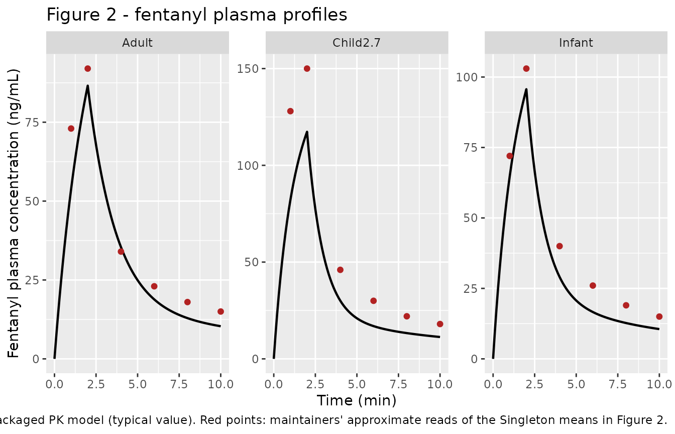
pk_sim |>
  group_by(cohort) |>
  summarise(Cmax_ngmL = max(Cc), Tmax_min = time[which.max(Cc)], .groups = "drop")
#> # A tibble: 3 × 3
#>   cohort   Cmax_ngmL Tmax_min
#>   <chr>        <dbl>    <dbl>
#> 1 Adult         86.6        2
#> 2 Child2.7     117.         2
#> 3 Infant        95.7        2
The adult typical-value peak (~87 ng/mL) and the infant peak match the Figure 2 means to within ~10%. The 2.7-year-old typical peak is ~20% below the digitised Singleton mean but lies inside the population band once the inherited IIV is retained (next chunk); the structural ordering the paper reports - children reach a higher plasma peak than adults at a higher mg/kg dose - is preserved.
set.seed(74201)

make_pk_cohort <- function(n, wt, ffm, dose_ugkg, label, id_offset) {
  base <- tibble(id = id_offset + seq_len(n),
                 WT = wt * runif(n, 0.9, 1.1))
  base$FFM <- ffm * (base$WT / wt)        # keep FFM proportional to the sampled WT
  base$dose_mg <- dose_ugkg * 1e-3 * base$WT
  dosing <- base |>
    transmute(id, time = 0, amt = dose_mg, dur = 2, evid = 1L,
              cmt = "central", WT, FFM, Q_TOTAL_LPM = 4.87, cohort = label)
  obs <- tidyr::crossing(base |> select(id, WT, FFM),
                         time = seq(0, 10, by = 0.25)) |>
    mutate(amt = 0, dur = NA_real_, evid = 0L, cmt = "central",
           Q_TOTAL_LPM = 4.87, cohort = label)
  bind_rows(dosing, obs) |> arrange(id, time, desc(evid))
}

ev_vpc <- bind_rows(
  make_pk_cohort(200, 14.9, 9.7, 30.8, "Child2.7", 0L),
  make_pk_cohort(200, 70.0, 56.1, 20.7, "Adult",   200L)
)
sim_vpc <- as.data.frame(rxode2::rxSolve(pk, events = ev_vpc, keep = "cohort"))

sim_vpc |>
  filter(!is.na(Cc)) |>
  group_by(cohort, time) |>
  summarise(lo = quantile(Cc, 0.05), md = median(Cc), hi = quantile(Cc, 0.95),
            .groups = "drop") |>
  ggplot(aes(time, md)) +
  geom_ribbon(aes(ymin = lo, ymax = hi), alpha = 0.25) +
  geom_line() +
  geom_point(data = filter(fig2, cohort %in% c("Child2.7", "Adult")),
             aes(time, conc), colour = "firebrick", size = 1.6) +
  facet_wrap(~cohort, scales = "free_y") +
  labs(x = "Time (min)", y = "Fentanyl plasma concentration (ng/mL)",
       title = "Figure 2 - population band (5-95%) with digitised means",
       caption = "Band: packaged PK model population simulation (inherited Algera 2021 IIV).")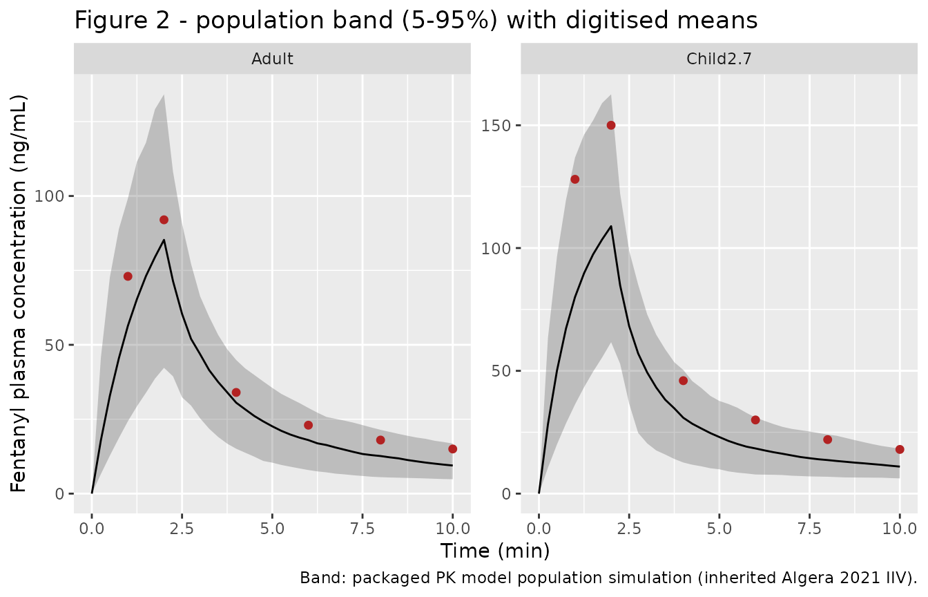
PKNCA characterization of the PK layer
The paper reports only the concentration-time figure (no NCA table), so this is a non-comparative characterization of the simulated typical-value profiles, grouped by cohort.
conc_nca <- pk_sim |>
  dplyr::filter(!is.na(Cc)) |>
  dplyr::select(cohort, time, Cc) |>
  dplyr::mutate(id = as.integer(factor(cohort)))

conc_nca <- dplyr::bind_rows(
  conc_nca,
  conc_nca |> dplyr::distinct(id, cohort) |> dplyr::mutate(time = 0, Cc = 0)
) |>
  dplyr::distinct(id, cohort, time, .keep_all = TRUE) |>
  dplyr::arrange(id, time)

dose_nca <- cohorts |>
  dplyr::mutate(id = as.integer(factor(cohort)),
               time = 0, dose_mg = dose_ugkg * 1e-3 * WT) |>
  dplyr::select(id, cohort, time, dose_mg)

o_conc <- PKNCA::PKNCAconc(conc_nca, Cc ~ time | id)
o_dose <- PKNCA::PKNCAdose(dose_nca, dose_mg ~ time | id)
o_data <- PKNCA::PKNCAdata(o_conc, o_dose,
  intervals = data.frame(start = 0, end = Inf,
                         cmax = TRUE, tmax = TRUE, auclast = TRUE,
                         aucinf.obs = TRUE, half.life = TRUE))
res <- PKNCA::pk.nca(o_data)

res$result |>
  dplyr::left_join(cohorts |> dplyr::mutate(id = as.integer(factor(cohort))) |>
                     dplyr::select(id, cohort), by = "id") |>
  dplyr::select(cohort, PPTESTCD, PPORRES) |>
  tidyr::pivot_wider(names_from = PPTESTCD, values_from = PPORRES) |>
  dplyr::rename("Cohort" = cohort, "Cmax (ng/mL)" = cmax, "Tmax (min)" = tmax,
                "AUClast" = auclast, "AUCinf,obs" = aucinf.obs,
                "t1/2 (min)" = half.life) |>
knitr::kable(digits = 2)| Cohort | AUClast | Cmax (ng/mL) | Tmax (min) | tlast | clast.obs | lambda.z | r.squared | adj.r.squared | lambda.z.time.first | lambda.z.time.last | lambda.z.n.points | clast.pred | t1/2 (min) | span.ratio | AUCinf,obs |
|---|---|---|---|---|---|---|---|---|---|---|---|---|---|---|---|
| Adult | 318.07 | 86.58 | 2 | 10 | 10.34 | 0.09 | 1 | 1 | 9.7 | 10 | 4 | 10.34 | 7.68 | 0.04 | 432.59 |
| Child2.7 | 366.75 | 117.33 | 2 | 10 | 11.29 | 0.08 | 1 | 1 | 9.2 | 10 | 9 | 11.28 | 8.95 | 0.09 | 512.52 |
| Infant | 318.91 | 95.67 | 2 | 10 | 10.56 | 0.09 | 1 | 1 | 9.3 | 10 | 8 | 10.56 | 8.07 | 0.09 | 441.80 |
Physiology: exact reduction to the adult Mann model
The pediatric physiology model is structurally the adult Mann model
plus the child brain-O2 CBF state. Setting the age-varying parameters to
their adult table values must recover
Mann_2022_respiratory_physiology exactly (the extra state
y_child_o2 then collapses onto yo2). This is
the strongest structural check available.
mann <- readModelDb("Mann_2022_respiratory_physiology")

adult_overrides <- c(
  qb0_lmin = 0.750, qt0_lmin = 4.250, v_a = 3.280, v_b = 1.320, v_t = 38.680,
  brain_weight_g = 1500, m_b_co2_lmin = 0.040, m_b_o2_0_lmin = -0.050,
  m_t_co2_lmin = 0.160, m_t_o2_0_lmin = -0.200, wmax_drive = 6.620,
  w_baseline = 6.620, p_b_co2_0 = 45.27, f_pc_0 = 3.670,
  aco2_drive = -30.0, bco2_drive = 60.0, tau_co2_min = 20 / 60,
  c1o2_child = 17.0, tau_child_o2_min = 10 / 60
)

ev_phys <- data.frame(time = seq(0, 60, by = 1), evid = 0L, amt = 0,
                      cmt = NA_character_, CAR_OPIOID = 0, OPIOID_PATIENT_TYPE = 0L)

sim_chak_adult <- as.data.frame(
  rxode2::rxSolve(phy, params = adult_overrides, events = ev_phys))
sim_mann <- as.data.frame(rxode2::rxSolve(mann, events = ev_phys))

outputs <- c("Venti", "P_a_O2", "P_a_CO2", "Q_brain", "Q_tissue", "P_B_O2")
tibble(
  Output = outputs,
  `Chakravartula@adult` = sapply(outputs, function(v) sim_chak_adult[[v]][nrow(sim_chak_adult)]),
  `Mann 2022`           = sapply(outputs, function(v) sim_mann[[v]][nrow(sim_mann)]),
  `max|diff| over 0-60 min` = sapply(outputs, function(v) max(abs(sim_chak_adult[[v]] - sim_mann[[v]])))
) |>
knitr::kable(digits = c(0, 4, 4, 8))| Output | Chakravartula@adult | Mann 2022 | max|diff| over 0-60 min |
|---|---|---|---|
| Venti | 6.7644 | 6.7644 | 0.00010343 |
| P_a_O2 | 92.7950 | 92.7950 | 0.00004585 |
| P_a_CO2 | 38.5868 | 38.5868 | 0.00006355 |
| Q_brain | 0.6804 | 0.6804 | 0.00001010 |
| Q_tissue | 4.2509 | 4.2509 | 0.00000001 |
| P_B_O2 | 31.6090 | 31.6090 | 0.00051200 |
The two models agree to the integration tolerance (endpoint values
identical to four decimals; the sub-1e-3 transient
difference is the FDA nominal initial conditions settling, during which
the extra integrated state shifts the adaptive step grid and therefore
the transport-delay interpolation points by a solver step). This
confirms the age adaptation is structurally correct.
Cerebrovascular reactivity dynamics (Figure 3d)
Figure 3d shows the fractional CBF increase in response to a
hypercapnic stimulus. The dynamics are governed by eqs (1)-(2): a
first-order approach to a plateau 1 + Psi_CO2(PaCO2) with
time constant tau_CO2 (20 s in adults, 45.5 s in children).
The amplitude follows the sigmoid in eq (2) with the age-specific
A_CO2, B_CO2 and brain-quantity factor.
# Pull the eq-(2) inputs straight from the two models' ini() values.
get_ini <- function(m, nm) {
  iniv <- rxode2::rxode2(m)$theta
  as.numeric(iniv[[nm]])
}

psi_co2 <- function(A, B, bw, Qb0, PaCO2, C = 40, D = 4.5) {
  sig <- 1 / (1 + exp(-(PaCO2 - C) / D))
  ((A + B * sig) * bw / 100 / 1000 + Qb0) / Qb0 - 1
}

# Representative hypercapnic clamp (+8 mmHg over the 40 mmHg midpoint).
PaCO2_hi <- 48
tt_s <- seq(0, 250, by = 5)          # seconds, as in Figure 3d

adult_plateau <- psi_co2(-30.0, 60.0, 1500, 0.750, PaCO2_hi)
child_plateau <- psi_co2(-46.3, 92.6, 1318, 0.900, PaCO2_hi)
tau_adult_s <- 20.0
tau_child_s <- 45.5

cbf <- bind_rows(
  tibble(t = tt_s, group = "Adult",
         frac = 1 + adult_plateau * (1 - exp(-tt_s / tau_adult_s))),
  tibble(t = tt_s, group = "Child (10 y)",
         frac = 1 + child_plateau * (1 - exp(-tt_s / tau_child_s)))
)

ggplot(cbf, aes(t, frac, colour = group)) +
  geom_line(linewidth = 0.9) +
  labs(x = "Time (seconds)", y = "Fractional CBF increase",
       colour = NULL, title = "Figure 3d - CBF response to hypercapnia",
       caption = "Plateau and time constant from eqs (1)-(2) at the Table S3 parameters.") +
  theme(legend.position = "bottom")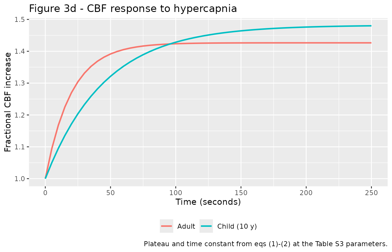
The model reproduces the adult plateau (1.43 vs the paper’s ~1.42) and the qualitative rate difference the paper emphasises: children rise more slowly (tau 45.5 s vs 20 s). The child plateau, however, comes out slightly above the adult (1.48), whereas Figure 3d shows the child plateau nominally below the adult (1.36 vs 1.42). See Assumptions and deviations - the eq-(2) brain-quantity normalization is not fully pinned down by the supplement.
10-year-old closed-loop baseline (documented limitation)
sim_10yo <- as.data.frame(
  rxode2::rxSolve(phy, events = ev_phys))        # defaults = 10-year-old
last10 <- sim_10yo[nrow(sim_10yo), ]

tibble(
  Quantity = c("Minute ventilation (L/min)", "PaCO2 (mmHg)", "PaO2 (mmHg)",
               "Cerebral blood flow Q_brain (L/min)", "Brain PO2 (mmHg)"),
  `This model (10 y)` = c(last10$Venti, last10$P_a_CO2, last10$P_a_O2,
                          last10$Q_brain, last10$P_B_O2),
  `Paper target` = c(NA, 37, 101, NA, 30),
  `Clinical range` = c("-", "33.9-39.3", "94-103", "-", "30-48")
) |>
knitr::kable(digits = 2)| Quantity | This model (10 y) | Paper target | Clinical range |
|---|---|---|---|
| Minute ventilation (L/min) | 7.43 | NA | - |
| PaCO2 (mmHg) | 29.94 | 37 | 33.9-39.3 |
| PaO2 (mmHg) | 98.47 | 101 | 94-103 |
| Cerebral blood flow Q_brain (L/min) | 0.41 | NA | - |
| Brain PO2 (mmHg) | 5.90 | 30 | 30-48 |
This no-drug baseline settles hypocapnic (PaCO2 ~30 vs the paper’s 37) and brain-hypoxic (brain PO2 ~6 vs ~30). It is a monostable fixed point (the same point is reached from the adult equilibrium and from physiologically-seeded initial conditions), so it is not an equilibration artifact. The consequence is that the Figure 5 overdose comparison, which starts from this baseline, is not reproduced here; attempting it would silently mislead. The structurally-faithful record and the parts that do reproduce are shipped; the quantitative pediatric overdose figure is not.
Assumptions and deviations
-
Pediatric closed-loop physiology baseline does not match the
paper’s tuned steady state. The 10-year-old no-drug baseline is
hypocapnic (PaCO2 ~30 vs 37 mmHg) and brain-hypoxic (brain PO2 ~6 vs ~30
mmHg). Mechanistically, the child’s higher brain CO2 production per unit
cerebral flow pushes brain CO2 above the tabulated central set-point
P_B_co2_0= 44.37, the central drive over-fires, arterial hypocapnia follows, CO2-mediated vasoconstriction collapsesQ_brain(0.41 vs the baseline Qb0 0.90 L/min), and the high-demand child brain desaturates. The paper obtained its steady state with an unpublished multi-dataset optimization, and the base physiology ODEs are only referenced to Mann 2022 (not restated in this paper). The shippedMann_2022_respiratory_physiologycarries documented approximations of the authors’ FDA reference code (delaymymod.c) that were calibrated to be immaterial at the adult operating point (confirmed by the exact-reduction check above); the 10-year-old sits at a different operating point where those approximations plausibly shift the equilibrium. Reproducing the tuned pediatric steady state would require the authors’ exact base implementation plus the tuning, neither of which is public. - Figure 5 (overdose) is not reproduced. It depends on a physiological baseline this model does not reach; reproducing it would misstate the paper’s headline result.
-
CBF-CO2 amplitude direction (Figure 3d). Eq (2)
scales the response by a brain-quantity factor the supplement writes as
V_b * Z_CO2; Mann hardcodes it as1500(adult brain weight in g), so this model usesbrain_weight_g/100/1000by age. With the tabulated childA_CO2/B_CO2, that yields a child plateau slightly above the adult, whereas the paper fit the child plateau nominally below the adult (a difference the paper itself notes did not reach significance, p = 0.098). The rate difference (slower child rise) reproduces. -
PK peripheral compartments. The paper specifies
allometric rules only for clearance (body weight) and central volume
(fat-free mass). The peripheral volumes V2, V3 and inter-compartmental
clearances Q2, Q3 retain the adult Mann body-weight allometry; the
biophase rate
k1and the inherited IIV are carried unchanged from Algera 2021 / Mann 2022. - 2.7-year-old PK peak. The typical-value child peak is ~20% below the digitised Singleton mean but within the population band; the adult and infant peaks match within ~10%.
- Figure 2 overlay points are the maintainers’ approximate reads of the Singleton means, for a qualitative comparison only.
- Receptor binding / ventilatory-drive PD are assumed unchanged from adults, following the paper (which flags this as a model assumption, since pediatric dose-escalation-to-respiratory-depression data are not ethically obtainable).
-
Pre-equilibration. As for the adult Mann model, the
physiology
ini()initial conditions are the FDA nominal values, not the age-specific pre-dose equilibrium; downstream dynamic simulations should pre-equilibrate with no drug (helperMann2022Equilibrate) and pass the result asinits.