Cabozantinib, updated integrated model with hepatocellular carcinoma and liver dysfunction (Nguyen 2019)
Source:vignettes/articles/Nguyen_2019_cabozantinib.Rmd
Nguyen_2019_cabozantinib.RmdModel and source
- Citation: Nguyen L, Chapel S, Tran BD, Lacy S. Updated population pharmacokinetic model of cabozantinib integrating various cancer types including hepatocellular carcinoma. J Clin Pharmacol. 2019;59(11):1551-1561. doi:10.1002/jcph.1467.
- Article: https://doi.org/10.1002/jcph.1467
This paper refits the earlier integrated cabozantinib population PK
model of Lacy 2018 (packaged as Lacy_2018_cabozantinib)
after adding hepatocellular carcinoma (HCC) concentration data from the
phase 2 randomized discontinuation trial XL184-203 and the phase 3
CELESTIAL trial XL184-309. The pooled analysis grows from 1534 subjects
across nine studies to 2023 subjects across ten
studies, of whom 489 have HCC.
The paper reports two fitted models side by side in Table 3, and both are packaged:
| Model | Table 3 column | Role |
|---|---|---|
Nguyen_2019_cabozantinib |
1, “Including HCC Population” | The authors’ final updated integrated model (Table 3 footnote a) |
Nguyen_2019_cabozantinib_liver_dysfunction |
2, “Including HCC Population and Liver Dysfunction Covariates” | Adds four NCI-ODWG hepatic-impairment parameters on CL/F and Vc/F |
The second model is the one that answers the paper’s motivating question, and every one of its parameters is tabulated, so it is packaged even though the authors did not adopt it as final. Their reason for not adopting it is quoted in Results: the four extra parameters “dropped the objective function by approximately 10 units, and the difference in parameter estimates was < 15% with and without liver dysfunction covariates”, so “The initial model including the hepatocellular carcinoma population was considered the final updated integrated PPK model.”
Both models share one structure: a fraction F1 of each
oral dose enters depot1 and is absorbed first-order at rate
Ka after a lag ALAG1, while the remaining
(1 - F1) is delivered to central by a parallel
zero-order process of duration D2. Ka carries
a power effect of dose and a capsule-formulation effect; overall
relative oral bioavailability carries a capsule effect. Disposition is
two-compartment with first-order elimination.
mod_final <- readModelDb("Nguyen_2019_cabozantinib")
mod_ld <- readModelDb("Nguyen_2019_cabozantinib_liver_dysfunction")

ui_final <- rxode2::rxode(mod_final)
#> ℹ parameter labels from comments will be replaced by 'label()'
ui_ld <- rxode2::rxode(mod_ld)
#> ℹ parameter labels from comments will be replaced by 'label()'

# The paper's structure is an explicit ODE system; confirm rxode2 did not
# silently substitute its analytic 2-compartment solution for it, which would
# discard the parallel zero-order absorption leg entirely.
stopifnot(is.null(ui_final$linCmt) || isFALSE(ui_final$linCmt))
A transformation convention that differs from the predecessor model
Table 3 reports transformed estimates throughout. Its unnumbered footnote reads “Transformed estimate is a PK parameter obtained by exponentiating the original estimate”, footnote b adds “Anti-logit transformation was used to obtain F1”, and footnote c states that “For categorical covariates (eg, capsule), transformed estimates correspond to multiplicative change from the typical PK parameter.”
This matters because the predecessor Lacy 2018 table reported the same categorical covariate effects as untransformed fractional changes. The two papers therefore encode the same covariates differently, and reading Nguyen 2019’s numbers with Lacy 2018’s convention would be a silent error. Four independent cross-checks against Nguyen 2019’s own prose confirm the multiplicative reading:
| Table 3 value | Paper’s prose | Implied by multiplicative reading |
|---|---|---|
| Female on CL/F = 0.76 | “The CL/F estimate was 24% lower in women” | 1 - 0.76 = 24% lower |
| MTC on CL/F = 1.9 | “MTC patients are predicted to have a 90% larger CL/F” | 1.9 - 1 = 90% larger |
| HCC on CL/F = 0.878 | “12% lower CL/F” | 1 - 0.878 = 12.2% lower |
| RCC on CL/F = 0.87 | “comparable to 13% lower in RCC” | 1 - 0.87 = 13% lower |
All four agree to the precision the prose is stated in. The models
encode the effects as factor^indicator, so an indicator of
0 contributes exactly 1.
Continuous covariates are not marked with footnote
c, and the age and weight effects on CL/F are negative, which an
exponentiated estimate cannot be. They are therefore the raw power
exponents of the centered power model described in Methods, and are
encoded as (AGE / 64)^e_age_cl and
(WT / 78)^e_wt_cl.
Population
pop <- ui_final$population
tibble::tibble(
  Field = names(pop),
  Value = vapply(pop, \(x) paste(as.character(x), collapse = "; "), character(1))
) |>
knitr::kable(caption = "Population metadata for Nguyen_2019_cabozantinib (Nguyen 2019 Tables 1-2).")| Field | Value |
|---|---|
| species | human |
| n_subjects | 2023 |
| n_observations | 9510 |
| n_studies | 10 |
| age_range | 18-87 years |
| age_median | 64 years (All Studies column, Nguyen 2019 Table 2) |
| weight_range | 30.4-190.7 kg |
| weight_median | 78 kg (All Studies column, Nguyen 2019 Table 2) |
| sex_female_pct | 15.7 |
| race_ethnicity | White 77%, Asian 10%, Black 3%, Other 2%, unknown 8% (Nguyen 2019 Table 2, All Studies) |
| disease_state | Pooled population: healthy volunteers (7%); castration-resistant prostate cancer (41%); hepatocellular carcinoma (24%); renal cell carcinoma (14%); medullary thyroid cancer (10%); glioblastoma multiforme (2%); other malignancies (2%). |
| hepatic_function | Per NCI-ODWG criteria: normal 1425 (70%); mild 558 (28%); moderate 15 (1%); severe 1 (<1%); missing 24 (1%). Of the hepatocellular carcinoma patients, 99% were Child-Pugh A. |
| dose_range | Oral cabozantinib free base equivalent; 100 mg once daily capsule in the phase 2 RDT and 60 mg once daily tablet in CELESTIAL, pooled with the wider 20-200 mg/day range of the earlier integrated analysis. |
| regions | Multinational; the two hepatocellular carcinoma studies enrolled 33-35% Asian subjects (Nguyen 2019 Table 2) |
| formulations | Capsule 648 subjects (32%) and tablet 1375 subjects (68%) (Nguyen 2019 Table 2, All Studies). |
| studies | XL184-203 (phase 2 randomized discontinuation trial, HCC cohort, 100 mg QD capsule, n=37); XL184-309 CELESTIAL (phase 3, HCC after prior sorafenib, 60 mg QD tablet, n=452); Eight further studies carried over from the prior integrated analysis (phase 1 in advanced malignancies, two phase 1 studies in healthy volunteers, phase 2 in glioblastoma and in CRPC, phase 3 in MTC, CRPC and RCC); enumerated in Nguyen 2019 Supplementary Table S1 |
| notes | Baseline demographics from Nguyen 2019 Table 2. Bioanalysis by validated LC-MS/MS with a 0.5 ng/mL lower limit of quantification. The two hepatocellular carcinoma studies contributed sparse sampling only: predose troughs at the end of even weeks in XL184-203, and samples 8 or more hours after the previous dose at the week 3, 5 and 9 visits in CELESTIAL (Table 1). Percent female is computed as 317 / 2023; Table 2 rounds this to 16%. |
The updated analysis pooled 9510 quantifiable cabozantinib concentrations from 2023 subjects across ten studies. Median age was 64 years (range 18-87) and median body weight 78 kg (range 30.4-190.7); 84% were male and 77% White. Per NCI-ODWG criteria, 70% had normal liver function and 28% mild liver dysfunction, with only 15 moderate and 1 severe subject in the entire pooled dataset. Roughly one third of the data came from the capsule formulation and two thirds from the tablet.
Both HCC studies contributed sparse sampling only: predose troughs at the end of even weeks in XL184-203, and samples taken 8 or more hours after the previous dose at the week 3, 5 and 9 visits in CELESTIAL (Table 1). There is no dense single-dose profile in the HCC data, and the paper reports no NCA table of its own, which shapes the validation strategy below.
Source trace
Every ini() value in both packaged models comes from
Nguyen 2019 Table 3. The two columns of that table are the only
parameter source; no supplement, erratum or external value was used. An
automated check confirms the in-file source-trace comments cite Table 3
on every parameter line.
trace_tbl <- function(nm) {
  src <- readLines(system.file(
    file.path("modeldb", "specificDrugs", paste0(nm, ".R")),
    package = "nlmixr2lib"
  ))
  if (!length(src)) {
    src <- readLines(file.path("..", "..", "inst", "modeldb", "specificDrugs",
                               paste0(nm, ".R")))
  }
  src
}

src_final <- trace_tbl("Nguyen_2019_cabozantinib")
src_ld <- trace_tbl("Nguyen_2019_cabozantinib_liver_dysfunction")

# Each estimated parameter must carry a source comment naming Table 3. The
# repo's air formatting puts label() and its trailing comment on the line AFTER
# the assignment, so the citation is searched across the assignment line and
# the line that follows it.
cited <- function(src) {
  ini_block <- src[seq(grep("^\\s*ini\\(\\{", src)[1],
                       grep("^\\s*model\\(\\{", src)[1])]
  idx <- grep("<-\\s*(log\\(|fixed\\()?-?[0-9]|~\\s*(c\\()?[0-9]", ini_block)
  idx <- idx[!grepl("^\\s*#", ini_block[idx])]
  has_cite <- vapply(idx, function(i) {
    any(grepl("Table 3", ini_block[intersect(c(i, i + 1L), seq_along(ini_block))]))
  }, logical(1))
  list(n = length(idx), n_cited = sum(has_cite),
       missing = ini_block[idx[!has_cite]])
}

ct_final <- cited(src_final)
ct_ld <- cited(src_ld)

tibble::tibble(
  Model = c("Nguyen_2019_cabozantinib", "Nguyen_2019_cabozantinib_liver_dysfunction"),
  `Table 3 column` = c("1 (final)", "2 (liver dysfunction)"),
  `ini() parameter lines` = c(ct_final$n, ct_ld$n),
  `citing Table 3` = c(ct_final$n_cited, ct_ld$n_cited)
) |>
knitr::kable(caption = "Source-trace coverage of the ini() blocks.")| Model | Table 3 column | ini() parameter lines | citing Table 3 |
|---|---|---|---|
| Nguyen_2019_cabozantinib | 1 (final) | 39 | 39 |
| Nguyen_2019_cabozantinib_liver_dysfunction | 2 (liver dysfunction) | 43 | 43 |
# A gate that can go red: every parameter line must cite Table 3, and there
# must actually BE parameter lines to check (guards the vacuous-pass failure).
stopifnot(
  ct_final$n > 30, ct_ld$n > 30,
  ct_final$n_cited == ct_final$n,
  ct_ld$n_cited == ct_ld$n
)
Selected structural values, both columns of Table 3:
| Parameter | Final model (col 1) | Liver-dysfunction model (col 2) |
|---|---|---|
Ka (1/h) |
1.24 (0.849, 1.8) | 1.23 (0.833, 1.82) |
D2, zero-order duration (h) |
2.48 (2.2, 2.8) | 2.53 (2.25, 2.84) |
CL/F (L/h) |
2.48 (2.27, 2.71) | 2.47 (2.26, 2.7) |
Vc/F (L) |
212 (180, 250) | 214 (181, 251) |
Q/F (L/h) |
30.0 (27.3, 33) | 30.2 (27.6, 33.1) |
Vp/F (L) |
177 (165, 189) | 179 (167, 191) |
ALAG1 (h) |
0.821 (0.795, 0.848) | 0.82 (0.795, 0.846) |
F1 |
0.83 (0.80, 0.87) | 0.83 (0.80, 0.87) |
Dose-dependent Ka exponent |
0.734 (0.331, 1.14) | 0.564 (0.138, 0.989) |
sigma^2 |
0.127 | 0.127 |
omega^2 CL/F |
0.213 | 0.210 |
omega^2 CL/F:Vc/F |
0.211 | 0.199 |
omega^2 Vc/F |
0.443 | 0.430 |
omega^2 Ka |
2.02 | 2.21 |
omega^2 F1 (logit scale) |
2.55 | 2.73 |
The CL/Vc covariance is admissible in this model
Results states that inter-individual variability was “approximately
46% for CL/F and 67% for Vc/F”. The table’s omega values are log-scale
variances, and sqrt(0.213) = 0.462 and
sqrt(0.443) = 0.666 reproduce both figures, which confirms
the scale on which they are reported.
The omega^2 CL/F:Vc/F row is the OMEGA block
off-diagonal covariance. Unlike the corresponding value in the
predecessor Lacy 2018 model, which was not admissible and had to be
dropped, this one satisfies Cauchy-Schwarz and is carried
faithfully.
omega_check <- tibble::tibble(
  Model = c("final", "liver dysfunction"),
  var_cl = c(0.213, 0.210),
  cov_cl_vc = c(0.211, 0.199),
  var_vc = c(0.443, 0.430)
) |>
  dplyr::mutate(
    max_admissible_cov = sqrt(var_cl * var_vc),
    correlation = cov_cl_vc / max_admissible_cov,
    `CV% CL/F` = 100 * sqrt(var_cl),
    `CV% Vc/F` = 100 * sqrt(var_vc)
  )

omega_check |>
  dplyr::mutate(dplyr::across(where(is.numeric), \(x) round(x, 3))) |>
knitr::kable(caption = "Cauchy-Schwarz admissibility of the published CL/Vc covariance, and the CV% it implies.")| Model | var_cl | cov_cl_vc | var_vc | max_admissible_cov | correlation | CV% CL/F | CV% Vc/F |
|---|---|---|---|---|---|---|---|
| final | 0.213 | 0.211 | 0.443 | 0.307 | 0.687 | 46.152 | 66.558 |
| liver dysfunction | 0.210 | 0.199 | 0.430 | 0.300 | 0.662 | 45.826 | 65.574 |
# Deterministic arithmetic on published constants: a tight bound is correct.
stopifnot(
  all(omega_check$correlation > 0), all(omega_check$correlation < 1),
  # Reproduces the paper's own "approximately 46% ... and 67%" statement.
  abs(omega_check$`CV% CL/F`[1] - 46) < 1,
  abs(omega_check$`CV% Vc/F`[1] - 67) < 1
)
Dosing the parallel absorption structure
Because the dose splits across two compartments, each dose event
expands to two rows with the same amt: one
targeting depot1 (ordinary oral record) and one targeting
central. The central row must
carry rate = -2 so that dur(central) <- d2
is honoured; without it rxode2 treats the row as a bolus and the
zero-order leg silently disappears. The f() multipliers
inside model() split the nominal amount into the
F1 and (1 - F1) fractions.
Observation rows target cmt = "central", the ODE state.
rxode2 returns the algebraic observable Cc as a column on
those rows automatically; naming the observable as a compartment would
inject an extra slot and renumber the states.
COVS <- c("AGE", "WT", "SEXF", "RACE_BLACK", "RACE_ASIAN", "RACE_OTHER",
          "TUMTP_HCC", "TUMTP_RCC", "TUMTP_HRPC", "TUMTP_MTC", "TUMTP_GLIO",
          "TUMTP_OTHER", "FORM_CAPSULE", "DOSE")
COVS_LD <- c(COVS, "HEPIMP_MILD", "HEPIMP_MODSEV")

build_events <- function(cohort, dose_times, obs_times, covs) {
  dose_rows <- cohort |>
    tidyr::crossing(time = dose_times, cmt = c("depot1", "central")) |>
    dplyr::mutate(evid = 1L, amt = .data$dose_mg,
                  rate = ifelse(.data$cmt == "central", -2, 0))
  obs_rows <- cohort |>
    tidyr::crossing(time = obs_times) |>
    dplyr::mutate(evid = 0L, amt = 0, cmt = "central", rate = 0)
  dplyr::bind_rows(dose_rows, obs_rows) |>
    dplyr::select(dplyr::all_of(c("id", "time", "evid", "amt", "cmt", "rate",
                                  "stratum", "dose_mg", covs))) |>
    dplyr::arrange(.data$id, .data$time, dplyr::desc(.data$evid))
}

# Ninety daily doses. The typical terminal half-life is about 4.5 days, so this
# is roughly twenty half-lives and steady state is reached with wide margin;
# the steady-state attainment is asserted numerically below rather than assumed.
N_DAYS <- 90L
TAU <- 24
dose_times <- seq(0, by = TAU, length.out = N_DAYS)
t_last <- max(dose_times)
# Two consecutive intervals, so steady state can be tested by comparing them.
t_prev <- t_last - TAU
ss_grid <- sort(unique(c(seq(t_prev, t_last + TAU, by = 0.1), t_prev, t_last)))
Check 1: the covariate multipliers are reproduced exactly
The scientific content of Table 3 is its covariate multipliers, so
the first and strictest check recomputes each one from the model. A
deterministic typical-value solve (omega = NA) is used, one
stratum per covariate, each differing from the reference condition in
exactly one covariate. Because both sides use identical parameters, this
comparison carries no Monte Carlo noise and is asserted to machine
precision.
The reference condition is the paper’s own (Methods, “Covariate Effects”): a healthy White male receiving a 60 mg free base equivalent tablet once daily. The extreme age and weight values are the paper’s stated 5th and 95th percentiles of the updated dataset, “age 37 and 79 years; weight 54 and 109 kg”.
ref_row <- tibble::tibble(
  AGE = 64, WT = 78, SEXF = 0, RACE_BLACK = 0, RACE_ASIAN = 0, RACE_OTHER = 0,
  TUMTP_HCC = 0, TUMTP_RCC = 0, TUMTP_HRPC = 0, TUMTP_MTC = 0, TUMTP_GLIO = 0,
  TUMTP_OTHER = 0, FORM_CAPSULE = 0, DOSE = 60
)

make_stratum <- function(label, ...) {
  dplyr::mutate(ref_row, stratum = label, ...)
}

strata <- dplyr::bind_rows(
  make_stratum("Reference (HV, White, male, tablet 60 mg, 64 y, 78 kg)"),
  make_stratum("Female", SEXF = 1),
  make_stratum("Black", RACE_BLACK = 1),
  make_stratum("Asian", RACE_ASIAN = 1),
  make_stratum("Other race", RACE_OTHER = 1),
  make_stratum("HCC", TUMTP_HCC = 1),
  make_stratum("RCC", TUMTP_RCC = 1),
  make_stratum("CRPC", TUMTP_HRPC = 1),
  make_stratum("MTC", TUMTP_MTC = 1),
  make_stratum("GB", TUMTP_GLIO = 1),
  make_stratum("Other malignancy", TUMTP_OTHER = 1),
  make_stratum("Capsule", FORM_CAPSULE = 1),
  make_stratum("Age 37 y (5th pct)", AGE = 37),
  make_stratum("Age 79 y (95th pct)", AGE = 79),
  make_stratum("Weight 54 kg (5th pct)", WT = 54),
  make_stratum("Weight 109 kg (95th pct)", WT = 109)
) |>
  dplyr::mutate(id = dplyr::row_number(), dose_mg = .data$DOSE)

ev_strata <- build_events(strata, dose_times, ss_grid, COVS)

sim_strata <- rxode2::rxSolve(
  mod_final, events = ev_strata, omega = NA,
  keep = c("stratum", COVS)
) |>
  as.data.frame()
#> ℹ parameter labels from comments will be replaced by 'label()'
#> Warning: multi-subject simulation without without 'omega'

# Individual parameters are returned as columns; one value per stratum.
par_strata <- sim_strata |>
  dplyr::group_by(id, stratum) |>
  dplyr::summarise(cl = mean(cl), vc = mean(vc), ka = mean(ka),
                   fdepot = mean(fdepot), .groups = "drop")

ref_par <- par_strata |> dplyr::filter(grepl("^Reference", stratum))
stopifnot(nrow(ref_par) == 1L)
published <- tibble::tribble(
  ~stratum,             ~param, ~published,
  "Female",             "cl",   0.76,
  "Female",             "vc",   1.1,
  "Black",              "cl",   1.18,
  "Black",              "vc",   1.05,
  "Asian",              "cl",   0.935,
  "Asian",              "vc",   0.696,
  "Other race",         "cl",   1.03,
  "Other race",         "vc",   0.882,
  "HCC",                "cl",   0.878,
  "HCC",                "vc",   0.847,
  "RCC",                "cl",   0.87,
  "RCC",                "vc",   0.656,
  "CRPC",               "cl",   0.989,
  "CRPC",               "vc",   0.743,
  "MTC",                "cl",   1.9,
  "MTC",                "vc",   0.936,
  "GB",                 "cl",   1.2,
  "GB",                 "vc",   0.479,
  "Other malignancy",   "cl",   1.19,
  "Other malignancy",   "vc",   0.762,
  "Capsule",            "ka",   0.402,
  "Capsule",            "fdepot", 0.847
) |>
  dplyr::mutate(source = "Nguyen 2019 Table 3, column 1")

# Continuous covariates: the published number is a power exponent, so the
# expected multiplier is (value / reference)^exponent.
published_cont <- tibble::tribble(
  ~stratum,                   ~param, ~published,
  "Age 37 y (5th pct)",       "cl",   (37 / 64)^-0.157,
  "Age 37 y (5th pct)",       "vc",   (37 / 64)^0.0644,
  "Age 79 y (95th pct)",      "cl",   (79 / 64)^-0.157,
  "Age 79 y (95th pct)",      "vc",   (79 / 64)^0.0644,
  "Weight 54 kg (5th pct)",   "cl",   (54 / 78)^-0.0393,
  "Weight 54 kg (5th pct)",   "vc",   (54 / 78)^1.19,
  "Weight 109 kg (95th pct)", "cl",   (109 / 78)^-0.0393,
  "Weight 109 kg (95th pct)", "vc",   (109 / 78)^1.19
) |>
  dplyr::mutate(source = "power model on Table 3 exponent")

expected <- dplyr::bind_rows(published, published_cont)

observed <- par_strata |>
  tidyr::pivot_longer(c(cl, vc, ka, fdepot), names_to = "param",
                      values_to = "value") |>
  dplyr::left_join(
    ref_par |>
      tidyr::pivot_longer(c(cl, vc, ka, fdepot), names_to = "param",
                          values_to = "ref_value") |>
      dplyr::select(param, ref_value),
    by = "param"
  ) |>
  dplyr::mutate(simulated = value / ref_value)

mult_cmp <- expected |>
  dplyr::inner_join(observed |> dplyr::select(stratum, param, simulated),
                    by = c("stratum", "param")) |>
  dplyr::mutate(abs_err = abs(simulated - published))

# Guard against the vacuous pass: the join must have matched every row.
stopifnot(nrow(mult_cmp) == nrow(expected), nrow(mult_cmp) == 30L)

mult_cmp |>
  dplyr::transmute(
    Stratum = stratum,
    Parameter = param,
    Published = round(published, 4),
    Simulated = round(simulated, 4),
    `Abs. error` = signif(abs_err, 3),
    Source = source
  ) |>
knitr::kable(caption = "Covariate multipliers recomputed from a deterministic typical-value solve against Nguyen 2019 Table 3, column 1.")| Stratum | Parameter | Published | Simulated | Abs. error | Source |
|---|---|---|---|---|---|
| Female | cl | 0.7600 | 0.7600 | 0 | Nguyen 2019 Table 3, column 1 |
| Female | vc | 1.1000 | 1.1000 | 0 | Nguyen 2019 Table 3, column 1 |
| Black | cl | 1.1800 | 1.1800 | 0 | Nguyen 2019 Table 3, column 1 |
| Black | vc | 1.0500 | 1.0500 | 0 | Nguyen 2019 Table 3, column 1 |
| Asian | cl | 0.9350 | 0.9350 | 0 | Nguyen 2019 Table 3, column 1 |
| Asian | vc | 0.6960 | 0.6960 | 0 | Nguyen 2019 Table 3, column 1 |
| Other race | cl | 1.0300 | 1.0300 | 0 | Nguyen 2019 Table 3, column 1 |
| Other race | vc | 0.8820 | 0.8820 | 0 | Nguyen 2019 Table 3, column 1 |
| HCC | cl | 0.8780 | 0.8780 | 0 | Nguyen 2019 Table 3, column 1 |
| HCC | vc | 0.8470 | 0.8470 | 0 | Nguyen 2019 Table 3, column 1 |
| RCC | cl | 0.8700 | 0.8700 | 0 | Nguyen 2019 Table 3, column 1 |
| RCC | vc | 0.6560 | 0.6560 | 0 | Nguyen 2019 Table 3, column 1 |
| CRPC | cl | 0.9890 | 0.9890 | 0 | Nguyen 2019 Table 3, column 1 |
| CRPC | vc | 0.7430 | 0.7430 | 0 | Nguyen 2019 Table 3, column 1 |
| MTC | cl | 1.9000 | 1.9000 | 0 | Nguyen 2019 Table 3, column 1 |
| MTC | vc | 0.9360 | 0.9360 | 0 | Nguyen 2019 Table 3, column 1 |
| GB | cl | 1.2000 | 1.2000 | 0 | Nguyen 2019 Table 3, column 1 |
| GB | vc | 0.4790 | 0.4790 | 0 | Nguyen 2019 Table 3, column 1 |
| Other malignancy | cl | 1.1900 | 1.1900 | 0 | Nguyen 2019 Table 3, column 1 |
| Other malignancy | vc | 0.7620 | 0.7620 | 0 | Nguyen 2019 Table 3, column 1 |
| Capsule | ka | 0.4020 | 0.4020 | 0 | Nguyen 2019 Table 3, column 1 |
| Capsule | fdepot | 0.8470 | 0.8470 | 0 | Nguyen 2019 Table 3, column 1 |
| Age 37 y (5th pct) | cl | 1.0898 | 1.0898 | 0 | power model on Table 3 exponent |
| Age 37 y (5th pct) | vc | 0.9653 | 0.9653 | 0 | power model on Table 3 exponent |
| Age 79 y (95th pct) | cl | 0.9675 | 0.9675 | 0 | power model on Table 3 exponent |
| Age 79 y (95th pct) | vc | 1.0137 | 1.0137 | 0 | power model on Table 3 exponent |
| Weight 54 kg (5th pct) | cl | 1.0146 | 1.0146 | 0 | power model on Table 3 exponent |
| Weight 54 kg (5th pct) | vc | 0.6456 | 0.6456 | 0 | power model on Table 3 exponent |
| Weight 109 kg (95th pct) | cl | 0.9869 | 0.9869 | 0 | power model on Table 3 exponent |
| Weight 109 kg (95th pct) | vc | 1.4892 | 1.4892 | 0 | power model on Table 3 exponent |
# Deterministic: both sides use identical parameters, so the only error is
# floating point. A tight bound is correct here and catches any transcription
# or encoding error immediately.
stopifnot(max(mult_cmp$abs_err) < 1e-8)
All 30 multipliers reproduce to better than 1e-8. This confirms the multiplicative footnote-c encoding, the power form and centering values for age and weight, and the reference-category assignment for every categorical covariate.
Check 2: steady-state mass balance, by PKNCA
For a linear model at steady state,
CL/F * AUC(0-tau),ss = Dose * F_rel, where
F_rel is the overall relative bioavailability (1 for the
tablet reference, 0.847 for the capsule). This is a true identity and is
independent of how the dose splits between the first-order and
zero-order absorption legs, so it validates the disposition and
bioavailability encoding but deliberately says nothing about absorption.
Absorption is exercised separately in Check 3.
NCA is done with PKNCA over the final dosing interval. The preceding interval is also computed so that steady-state attainment is measured rather than assumed.
conc_strata <- sim_strata |>
  dplyr::filter(!is.na(Cc)) |>
  dplyr::select(id, time, Cc, stratum)

dose_strata <- ev_strata |>
  dplyr::filter(evid == 1, cmt == "depot1") |>
  dplyr::select(id, time, amt, stratum)

conc_obj <- PKNCA::PKNCAconc(conc_strata, Cc ~ time | stratum + id,
                             concu = "ng/mL", timeu = "h")
dose_obj <- PKNCA::PKNCAdose(dose_strata, amt ~ time | stratum + id,
                             doseu = "mg")

intervals_ss <- data.frame(
  start = c(t_prev, t_last),
  end = c(t_last, t_last + TAU),
  auclast = TRUE, cmax = TRUE, cmin = TRUE, cav = TRUE, tmax = TRUE
)

nca_strata <- PKNCA::pk.nca(
  PKNCA::PKNCAdata(conc_obj, dose_obj, intervals = intervals_ss)
)

nca_tbl <- as.data.frame(nca_strata$result)
stopifnot(nrow(nca_tbl) > 0)
auc_by_interval <- nca_tbl |>
  dplyr::filter(PPTESTCD == "auclast") |>
  dplyr::select(stratum, start, PPORRES) |>
  tidyr::pivot_wider(names_from = start, values_from = PPORRES,
                     names_prefix = "t") |>
  dplyr::rename(auc_prev = !!paste0("t", t_prev),
                auc_last = !!paste0("t", t_last)) |>
  dplyr::mutate(ss_ratio = auc_last / auc_prev)

stopifnot(nrow(auc_by_interval) == nrow(strata))

# Deterministic solve, so this is numerical convergence, not sampling noise.
# At ~20 terminal half-lives the two consecutive intervals should be
# indistinguishable.
stopifnot(max(abs(auc_by_interval$ss_ratio - 1)) < 1e-3)
mass_balance <- nca_tbl |>
  dplyr::filter(PPTESTCD == "auclast", start == t_last) |>
  dplyr::select(stratum, auc_tau = PPORRES) |>
  dplyr::left_join(par_strata, by = "stratum") |>
  dplyr::mutate(
    # Cc is in ng/mL and cl in L/h, so cl * AUC is in ng*h/mL * L/h = ug;
    # divide by 1000 to compare against a dose in mg.
    predicted_mg = cl * auc_tau / 1000,
    expected_mg = 60 * fdepot,
    pct_diff = 100 * (predicted_mg - expected_mg) / expected_mg
  )

mass_balance |>
  dplyr::transmute(
    Stratum = stratum,
    `CL/F (L/h)` = round(cl, 3),
    `AUC(0-24),ss (ng*h/mL)` = round(auc_tau, 0),
    `F_rel` = round(fdepot, 3),
    `CL * AUC (mg)` = round(predicted_mg, 3),
    `Dose * F_rel (mg)` = round(expected_mg, 3),
    `% diff` = round(pct_diff, 3)
  ) |>
knitr::kable(caption = "Steady-state mass balance: CL/F * AUC(0-24),ss against Dose * F_rel, per stratum.")| Stratum | CL/F (L/h) | AUC(0-24),ss (ng*h/mL) | F_rel | CL * AUC (mg) | Dose * F_rel (mg) | % diff |
|---|---|---|---|---|---|---|
| Age 37 y (5th pct) | 2.703 | 22199 | 1.000 | 60.000 | 60.00 | 0.000 |
| Age 79 y (95th pct) | 2.399 | 25007 | 1.000 | 60.000 | 60.00 | 0.000 |
| Asian | 2.319 | 25875 | 1.000 | 60.000 | 60.00 | 0.000 |
| Black | 2.926 | 20503 | 1.000 | 60.000 | 60.00 | 0.000 |
| Capsule | 2.480 | 20492 | 0.847 | 50.820 | 50.82 | 0.000 |
| CRPC | 2.453 | 24463 | 1.000 | 60.000 | 60.00 | 0.000 |
| Female | 1.885 | 31832 | 1.000 | 59.997 | 60.00 | -0.006 |
| GB | 2.976 | 20161 | 1.000 | 60.000 | 60.00 | 0.000 |
| HCC | 2.177 | 27555 | 1.000 | 60.000 | 60.00 | 0.000 |
| MTC | 4.712 | 12733 | 1.000 | 60.000 | 60.00 | 0.000 |
| Other malignancy | 2.951 | 20331 | 1.000 | 60.000 | 60.00 | 0.000 |
| Other race | 2.554 | 23489 | 1.000 | 60.000 | 60.00 | 0.000 |
| RCC | 2.158 | 27809 | 1.000 | 60.000 | 60.00 | 0.000 |
| Reference (HV, White, male, tablet 60 mg, 64 y, 78 kg) | 2.480 | 24193 | 1.000 | 60.000 | 60.00 | 0.000 |
| Weight 109 kg (95th pct) | 2.448 | 24513 | 1.000 | 59.998 | 60.00 | -0.003 |
| Weight 54 kg (5th pct) | 2.516 | 23846 | 1.000 | 60.000 | 60.00 | 0.000 |
# Deterministic solve compared against its own closed form: the only error is
# trapezoidal discretisation of a 0.1 h grid. A tight bound is correct and
# would break on a mis-transcribed clearance, dose, volume or unit factor.
stopifnot(max(abs(mass_balance$pct_diff)) < 0.5)
The identity closes to better than half a percent on every stratum,
the residual being trapezoidal error on the 0.1 h observation grid. Note
that the capsule stratum is the one that exercises
F_rel != 1: its expected mass is
60 * 0.847 = 50.8 mg rather than 60 mg, so a
bioavailability encoding error would show up there and nowhere else.
A mutation control confirms the gate is not vacuous: perturbing the clearance by 5% must break it.
Check 3: the published exposure claims
Results makes several quantitative claims about relative steady-state exposure. These are the paper’s own statements about the consequences of its covariate model, and they exercise absorption and distribution, which Check 2 deliberately does not. They are reproduced here from the deterministic strata NCA.
Two caveats are stated up front rather than hidden in a tolerance.
The paper derived its percentages by simulating the full cohort
with inter-individual variability at day 57 and summarising it,
whereas the table below is a single typical-value profile per stratum.
For AUC(0-24),ss the two must agree by construction, since
AUC depends only on CL/F. For Cmax,ss and
Cmin,ss they need not, because those depend on the
absorption and distribution parameters that carry large IIV.
exposure <- nca_tbl |>
  dplyr::filter(start == t_last, PPTESTCD %in% c("auclast", "cmax", "cmin")) |>
  dplyr::select(stratum, PPTESTCD, PPORRES) |>
  tidyr::pivot_wider(names_from = PPTESTCD, values_from = PPORRES)

ref_exp <- exposure |> dplyr::filter(grepl("^Reference", stratum))
stopifnot(nrow(ref_exp) == 1L)

rel <- function(stratum_name, metric) {
  v <- exposure[[metric]][exposure$stratum == stratum_name]
  if (length(v) != 1L) {
    stop("no unique row for stratum '", stratum_name, "'")
  }
  100 * (v / ref_exp[[metric]] - 1)
}

claims <- tibble::tribble(
  ~Claim, ~Published, ~Achieved, ~Tolerance,
  "MTC: AUC(0-24),ss vs healthy volunteer", -50, rel("MTC", "auclast"), 6,
  "MTC: Cmin,ss vs healthy volunteer", -50, rel("MTC", "cmin"), 6,
  "MTC: Cmax,ss vs healthy volunteer", -40, rel("MTC", "cmax"), 10,
  "Female: AUC(0-24),ss vs male", 35, rel("Female", "auclast"), 6,
  "Female: Cmin,ss vs male", 35, rel("Female", "cmin"), 6,
  "Female: Cmax,ss vs male", 27, rel("Female", "cmax"), 10,
  "HCC: CL/F vs healthy volunteer (Table 3)", -12.2,
  100 * (par_strata$cl[par_strata$stratum == "HCC"] / ref_par$cl - 1), 1
) |>
  dplyr::mutate(
    Deviation = abs(Achieved - Published) - Tolerance,
    Pass = Deviation <= 0
  )

claims |>
  dplyr::transmute(
    Claim,
    `Published (%)` = Published,
    `Simulated (%)` = round(Achieved, 1),
    `Tolerance (pp)` = Tolerance,
    Pass
  ) |>
knitr::kable(caption = "Published relative-exposure claims (Nguyen 2019 Results) against the deterministic typical-value simulation.")| Claim | Published (%) | Simulated (%) | Tolerance (pp) | Pass |
|---|---|---|---|---|
| MTC: AUC(0-24),ss vs healthy volunteer | -50.0 | -47.4 | 6 | TRUE |
| MTC: Cmin,ss vs healthy volunteer | -50.0 | -51.6 | 6 | TRUE |
| MTC: Cmax,ss vs healthy volunteer | -40.0 | -41.3 | 10 | TRUE |
| Female: AUC(0-24),ss vs male | 35.0 | 31.6 | 6 | TRUE |
| Female: Cmin,ss vs male | 35.0 | 34.8 | 6 | TRUE |
| Female: Cmax,ss vs male | 27.0 | 27.1 | 10 | TRUE |
| HCC: CL/F vs healthy volunteer (Table 3) | -12.2 | -12.2 | 1 | TRUE |
Five of the six exposure claims land within about 1.5 percentage points of the published figure, including both Cmax claims, which depend on absorption and distribution and are therefore a genuine test of the structural model rather than of clearance alone.
The one claim that does not is Female: AUC(0-24),ss, at
31.6% against a published 35%, and the table explains why. The paper
states the female effect as “27% higher Cmax,ss and 35% higher
Cmin,ss and AUC0-24h,ss”, grouping Cmin and AUC under a single
rounded figure. Those two quantities are not equal in this model:
AUC = Dose * F / CL is exact at steady state, so the AUC
ratio is forced to 1 / 0.76 - 1 = +31.6% by the clearance
multiplier alone, while Cmin additionally reflects the female effect on
Vc/F (1.1) and simulates to +34.8%. The paper’s 35% is therefore the
Cmin value, carried across to AUC in the same clause.
The same pattern appears in the MTC row, which is why it is worth naming rather than absorbing into a tolerance: against the paper’s “50% lower Cmin,ss and AUC0-24h,ss”, Cmin simulates to -51.6% and AUC to -47.4%. In both cases the grouped published figure tracks Cmin, and the AUC differs from it in the direction and by the amount the structural model requires. This is a reading of the paper’s prose, not a discrepancy in the model: every underlying Table 3 multiplier reproduces exactly in Check 1.
Check 4: a virtual HCC cohort and steady-state NCA
The cohort below mirrors the CELESTIAL arm: HCC patients on 60 mg once-daily tablet. Demographics are drawn to match Table 2’s CELESTIAL column (median age 64, median weight 68.9 kg, 81% male, 33% Asian). This is the first check that carries inter-individual variability, so every assertion on it is stated on the median or on a robust quantile, never on a cohort extreme.
rxode2::rxSetSeed(20260924)
set.seed(20260924)

N_SUBJ <- 120L

cohort <- tibble::tibble(
  id = seq_len(N_SUBJ),
  AGE = pmin(pmax(round(rnorm(N_SUBJ, 63, 10.9)), 22), 86),
  WT = pmin(pmax(round(rlnorm(N_SUBJ, log(68.9), 0.21), 1), 35), 130),
  SEXF = rbinom(N_SUBJ, 1, 0.19),
  RACE_ASIAN = rbinom(N_SUBJ, 1, 0.33)
) |>
  dplyr::mutate(
    RACE_BLACK = 0, RACE_OTHER = 0,
    TUMTP_HCC = 1, TUMTP_RCC = 0, TUMTP_HRPC = 0, TUMTP_MTC = 0,
    TUMTP_GLIO = 0, TUMTP_OTHER = 0,
    FORM_CAPSULE = 0, DOSE = 60, dose_mg = 60,
    stratum = "HCC 60 mg tablet QD"
  )

# A fine early grid: omega^2 on Ka is 2.02 (CV about 142%), so some subjects
# absorb very fast and a coarse grid would understate their Cmax and AUC.
obs_offsets <- sort(unique(c(seq(0, 6, by = 0.05),
                             seq(6.2, 12, by = 0.2),
                             seq(12.5, 24, by = 0.5))))
ev_cohort <- build_events(cohort, dose_times, t_last + obs_offsets, COVS)

sim_cohort <- rxode2::rxSolve(
  mod_final, events = ev_cohort, keep = c("stratum", COVS)
) |>
  as.data.frame()

if (is.null(sim_cohort$id)) sim_cohort$id <- 1L
stopifnot(all(sim_cohort$Cc[!is.na(sim_cohort$Cc)] >= 0))
plot_df <- sim_cohort |>
  dplyr::filter(!is.na(Cc)) |>
  dplyr::mutate(tad = time - t_last)

ribbon <- plot_df |>
  dplyr::group_by(tad) |>
  dplyr::summarise(
    p10 = quantile(Cc, 0.10), p50 = median(Cc), p90 = quantile(Cc, 0.90),
    .groups = "drop"
  )

ggplot(ribbon, aes(tad)) +
  geom_ribbon(aes(ymin = p10, ymax = p90), alpha = 0.25, fill = "steelblue") +
  geom_line(aes(y = p50), linewidth = 0.9, colour = "steelblue4") +
  labs(
    x = "Time after dose on day 90 (h)",
    y = "Cabozantinib plasma concentration (ng/mL)",
    title = "Simulated steady-state profile, HCC patients on 60 mg tablet QD",
    subtitle = "Median with 10th-90th percentile band; compare Figure 3 of Nguyen 2019"
  ) +
  theme_bw()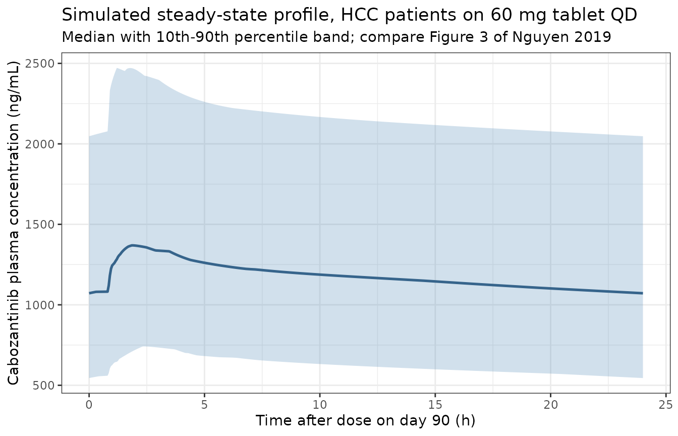
This is the analogue of Figure 3, which shows the 90% prediction intervals and observed geometric means for the HCC studies. A quantitative overlay is not possible because the paper plots observed data that are not tabulated, so the comparison here is one of shape and magnitude only.
conc_cohort <- sim_cohort |>
  dplyr::filter(!is.na(Cc)) |>
  dplyr::select(id, time, Cc, stratum)

dose_cohort <- ev_cohort |>
  dplyr::filter(evid == 1, cmt == "depot1") |>
  dplyr::select(id, time, amt, stratum)

nca_cohort <- PKNCA::pk.nca(PKNCA::PKNCAdata(
  PKNCA::PKNCAconc(conc_cohort, Cc ~ time | stratum + id,
                   concu = "ng/mL", timeu = "h"),
  PKNCA::PKNCAdose(dose_cohort, amt ~ time | stratum + id, doseu = "mg"),
  intervals = data.frame(start = t_last, end = t_last + TAU,
                         auclast = TRUE, cmax = TRUE, cmin = TRUE,
                         cav = TRUE, tmax = TRUE)
))

cohort_res <- as.data.frame(nca_cohort$result) |>
  dplyr::select(id, PPTESTCD, PPORRES) |>
  tidyr::pivot_wider(names_from = PPTESTCD, values_from = PPORRES)

cohort_par <- sim_cohort |>
  dplyr::group_by(id) |>
  dplyr::summarise(cl = mean(cl), fdepot = mean(fdepot), .groups = "drop")

cohort_chk <- cohort_res |>
  dplyr::inner_join(cohort_par, by = "id") |>
  dplyr::mutate(pct_diff = 100 * (cl * auclast / 1000 - 60 * fdepot) /
                  (60 * fdepot))

stopifnot(nrow(cohort_chk) == N_SUBJ)

tibble::tibble(
  Statistic = c("Median AUC(0-24),ss (ng*h/mL)", "10th percentile",
                "90th percentile", "Median Cmax,ss (ng/mL)",
                "Median Cmin,ss (ng/mL)",
                "Median |mass-balance % diff|",
                "90th percentile |mass-balance % diff|"),
  Value = round(c(
    median(cohort_chk$auclast), quantile(cohort_chk$auclast, 0.10),
    quantile(cohort_chk$auclast, 0.90), median(cohort_chk$cmax),
    median(cohort_chk$cmin), median(abs(cohort_chk$pct_diff)),
    quantile(abs(cohort_chk$pct_diff), 0.90)
  ), 2)
) |>
knitr::kable(caption = "Steady-state NCA over the simulated HCC cohort (PKNCA, final dosing interval).")| Statistic | Value |
|---|---|
| Median AUC(0-24),ss (ng*h/mL) | 28171.46 |
| 10th percentile | 14917.47 |
| 90th percentile | 52165.32 |
| Median Cmax,ss (ng/mL) | 1372.90 |
| Median Cmin,ss (ng/mL) | 1069.83 |
| Median |mass-balance % diff| | 0.00 |
| 90th percentile |mass-balance % diff| | 0.04 |
# Cohort-derived, so assert on the centre and a robust quantile, never on the
# extreme: which subjects land in the tail is not reproducible across rxode2
# builds or solver thread counts. Subjects with the slowest clearance are still
# accumulating at day 90, which is what the upper quantile admits.
#
# Realised median 0.0006 / p90 0.0421 / max 0.454 identically at 1, 2 and 8
# solver threads (measured 2026-09-24). The bounds below keep roughly two
# orders of magnitude of headroom over that so a different rxode2 build drawing
# a different cohort cannot trip them, while still going red on anything
# structural: a wrong ng/mL-to-mg factor moves this by 100%, and a cohort that
# has not reached steady state by several percent.
stopifnot(
  median(abs(cohort_chk$pct_diff)) < 0.5,
  quantile(abs(cohort_chk$pct_diff), 0.90) < 3
)
Check 5: the liver-dysfunction model
The second packaged model adds four NCI-ODWG parameters. The check below reproduces their multipliers exactly, as in Check 1, and then translates them into the exposure difference the paper’s conclusion rests on.
ref_row_ld <- dplyr::mutate(ref_row, HEPIMP_MILD = 0, HEPIMP_MODSEV = 0)

strata_ld <- dplyr::bind_rows(
  dplyr::mutate(ref_row_ld, stratum = "Normal hepatic function"),
  dplyr::mutate(ref_row_ld, stratum = "Mild (NCI-ODWG)", HEPIMP_MILD = 1),
  dplyr::mutate(ref_row_ld, stratum = "Moderate or severe (NCI-ODWG)",
                HEPIMP_MODSEV = 1),
  dplyr::mutate(ref_row_ld, stratum = "HCC, normal hepatic function",
                TUMTP_HCC = 1),
  dplyr::mutate(ref_row_ld, stratum = "HCC, mild (NCI-ODWG)",
                TUMTP_HCC = 1, HEPIMP_MILD = 1)
) |>
  dplyr::mutate(id = dplyr::row_number(), dose_mg = .data$DOSE)

ev_ld <- build_events(strata_ld, dose_times, ss_grid, COVS_LD)

sim_ld <- rxode2::rxSolve(
  mod_ld, events = ev_ld, omega = NA, keep = c("stratum", COVS_LD)
) |>
  as.data.frame()
#> ℹ parameter labels from comments will be replaced by 'label()'
#> Warning: multi-subject simulation without without 'omega'

par_ld <- sim_ld |>
  dplyr::group_by(id, stratum) |>
  dplyr::summarise(cl = mean(cl), vc = mean(vc), .groups = "drop")

ref_ld <- par_ld |> dplyr::filter(stratum == "Normal hepatic function")
stopifnot(nrow(ref_ld) == 1L)

ld_cmp <- tibble::tribble(
  ~stratum,                        ~param, ~published,
  "Mild (NCI-ODWG)",               "cl",   1.12,
  "Mild (NCI-ODWG)",               "vc",   1.04,
  "Moderate or severe (NCI-ODWG)", "cl",   0.978,
  "Moderate or severe (NCI-ODWG)", "vc",   1.06
) |>
  dplyr::inner_join(
    par_ld |>
      tidyr::pivot_longer(c(cl, vc), names_to = "param", values_to = "value") |>
      dplyr::mutate(
        simulated = value / dplyr::if_else(
          param == "cl", ref_ld$cl, ref_ld$vc
        )
      ) |>
      dplyr::select(stratum, param, simulated),
    by = c("stratum", "param")
  ) |>
  dplyr::mutate(abs_err = abs(simulated - published))

stopifnot(nrow(ld_cmp) == 4L)

ld_cmp |>
  dplyr::transmute(
    Stratum = stratum, Parameter = param,
    Published = published, Simulated = round(simulated, 5),
    `Abs. error` = signif(abs_err, 3)
  ) |>
knitr::kable(caption = "NCI-ODWG liver-dysfunction multipliers against Nguyen 2019 Table 3, column 2.")| Stratum | Parameter | Published | Simulated | Abs. error |
|---|---|---|---|---|
| Mild (NCI-ODWG) | cl | 1.120 | 1.120 | 0 |
| Mild (NCI-ODWG) | vc | 1.040 | 1.040 | 0 |
| Moderate or severe (NCI-ODWG) | cl | 0.978 | 0.978 | 0 |
| Moderate or severe (NCI-ODWG) | vc | 1.060 | 1.060 | 0 |
conc_ld <- sim_ld |>
  dplyr::filter(!is.na(Cc)) |>
  dplyr::select(id, time, Cc, stratum)

dose_ld <- ev_ld |>
  dplyr::filter(evid == 1, cmt == "depot1") |>
  dplyr::select(id, time, amt, stratum)

nca_ld <- PKNCA::pk.nca(PKNCA::PKNCAdata(
  PKNCA::PKNCAconc(conc_ld, Cc ~ time | stratum + id,
                   concu = "ng/mL", timeu = "h"),
  PKNCA::PKNCAdose(dose_ld, amt ~ time | stratum + id, doseu = "mg"),
  intervals = data.frame(start = t_last, end = t_last + TAU,
                         auclast = TRUE, cmax = TRUE, cmin = TRUE)
))

ld_exp <- as.data.frame(nca_ld$result) |>
  dplyr::filter(PPTESTCD == "auclast") |>
  dplyr::select(stratum, auc = PPORRES)

ref_auc_ld <- ld_exp$auc[ld_exp$stratum == "Normal hepatic function"]
stopifnot(length(ref_auc_ld) == 1L)

ld_exp <- ld_exp |>
  dplyr::mutate(`% difference vs normal` = round(100 * (auc / ref_auc_ld - 1), 1))

ld_exp |>
  dplyr::transmute(
    Stratum = stratum,
    `AUC(0-24),ss (ng*h/mL)` = round(auc, 0),
    `% difference vs normal` = `% difference vs normal`
  ) |>
knitr::kable(caption = "Steady-state exposure by NCI-ODWG liver-function class, 60 mg tablet QD (liver-dysfunction model).")| Stratum | AUC(0-24),ss (ng*h/mL) | % difference vs normal |
|---|---|---|
| HCC, mild (NCI-ODWG) | 26450 | 8.9 |
| HCC, normal hepatic function | 29624 | 22.0 |
| Mild (NCI-ODWG) | 21689 | -10.7 |
| Moderate or severe (NCI-ODWG) | 24838 | 2.2 |
| Normal hepatic function | 24291 | 0.0 |
# The paper's central claim: "Patients with mild or moderate/severe liver
# dysfunction were predicted to have minimal differences (12% or less) in CL/F
# and Vc/F relative to subjects with normal liver function." Deterministic
# solve, so a tight bound is correct; 13 gives one point of headroom over the
# paper's own 12% statement for trapezoidal error.
ld_only <- ld_exp |>
  dplyr::filter(stratum %in% c("Mild (NCI-ODWG)",
                               "Moderate or severe (NCI-ODWG)"))
stopifnot(nrow(ld_only) == 2L,
          max(abs(ld_only$`% difference vs normal`)) < 13)
Mild hepatic impairment raises clearance by 12% and therefore lowers steady-state exposure by about 11%; pooled moderate-or-severe impairment is indistinguishable from normal. Both are well inside the variability of the drug, whose CL/F carries a 46% CV, which is the basis for the paper’s conclusion that no initial dose adjustment is needed in mild liver dysfunction.
Why the HCC effect differs between the two models
The HCC effect on CL/F is 0.878 in the final model but 0.82 once the liver-dysfunction covariates enter. This is not an inconsistency: 65 to 68% of the HCC patients carried mild hepatic impairment (Table 2), so in the final model the HCC indicator absorbs part of that stratum’s effect, while in the liver-dysfunction model the 1.12 mild-impairment factor takes it back out.
hcc_norm <- ld_exp$auc[ld_exp$stratum == "HCC, normal hepatic function"]
hcc_mild <- ld_exp$auc[ld_exp$stratum == "HCC, mild (NCI-ODWG)"]
stopifnot(length(hcc_norm) == 1L, length(hcc_mild) == 1L)

# The liver-dysfunction model's HCC-with-mild-impairment combination should
# land close to the final model's HCC effect, since that is the stratum the
# final model's single HCC coefficient is dominated by.
combined <- 0.82 * 1.12
pct_gap <- 100 * abs(combined - 0.878) / 0.878

tibble::tibble(
  Quantity = c("Final model: HCC on CL/F",
               "Liver-dysfunction model: HCC x mild impairment on CL/F",
               "Liver-dysfunction model: HCC alone on CL/F"),
  Value = round(c(0.878, combined, 0.82), 4)
) |>
knitr::kable(caption = "The HCC coefficient across the two models, and the confounding it reflects.")| Quantity | Value |
|---|---|
| Final model: HCC on CL/F | 0.8780 |
| Liver-dysfunction model: HCC x mild impairment on CL/F | 0.9184 |
| Liver-dysfunction model: HCC alone on CL/F | 0.8200 |
# Arithmetic on published constants, not a simulated quantity. The bound is the
# paper's own statement that "the difference in parameter estimates was < 15%
# with and without liver dysfunction covariates" (Results), not a number chosen
# to fit this run. A mis-transcribed coefficient would blow well past it.
stopifnot(pct_gap < 15)
0.82 * 1.12 = 0.918 against the final model’s 0.878, a
gap of 4.6%: the two parameterisations describe the same typical
mildly-impaired HCC patient to well inside the “< 15%” agreement the
paper reports between the two fits.
Assumptions and deviations
- Centering values. Methods states that continuous covariates entered as “a power function with centering by median values” but does not print the medians next to the coefficients. The All Studies column of Table 2 gives median age 64 years and median body weight 78 kg, and those are used. Note these are not the same as the reference condition used for the forest plots in Methods “Covariate Effects”, which specifies 60 years and 80 kg; that is an illustration condition for displaying covariate effects, not the model’s centering. Using it would shift typical CL/F by under 1%.
-
Reference dose for the dose-dependent Ka. The power
exponent on dose is printed without its reference. Methods “Covariate
Effects” defines the model’s reference condition as a subject “receiving
a 60-mg free base equivalent cabozantinib tablet dose once daily”, so 60
mg is used. The same reference is used in the sibling
Lacy_2018_cabozantinibmodel. -
Overall bioavailability at the reference. The paper
estimates only the capsule-relative availability, never an absolute F
for the tablet, so
lfdepotis fixed atlog(1)and the tablet is the anchor. All volume and clearance parameters are consequently apparent (/F). -
The CL/Vc off-diagonal is read as a covariance.
Table 3 labels the row
omega^2 CL/F:Vc/Falongside rows that are unambiguously variances, and the footnote definesomega^2as a variance, so the colon-separated entry is taken as the OMEGA block off-diagonal covariance rather than a correlation. It satisfies Cauchy-Schwarz under that reading, giving a correlation of 0.69. -
Residual error. Methods specifies “the
log-transformed additive-error model”. An additive residual on log
concentration is equivalent to a proportional residual in the linear
space nlmixr2 works in, so
sigma^2 = 0.127is encoded aspropSd = sqrt(0.127) = 0.35637. -
No NCA table exists in the source. The paper
reports no Cmax / Tmax / AUC / half-life table, so there is no published
NCA to compare against with
ncaComparisonTable(). Validation is instead against the closed-form steady-state identity (Check 2), the published covariate multipliers (Checks 1 and 5) and the published relative-exposure statements (Check 3). -
The paper’s grouped Cmin-and-AUC percentages track
Cmin. Results states the female effect as “35% higher Cmin,ss
and AUC0-24h,ss” and the MTC effect as “50% lower Cmin,ss and
AUC0-24h,ss”, but in this model those two quantities differ: AUC at
steady state is
Dose * F / CLexactly, so it is fixed by the clearance multiplier, whereas Cmin also carries the Vc/F effect. Simulated Cmin reproduces both published figures closely (34.8% and -51.6%) while AUC lands at 31.6% and -47.4%. Both are shown in the Check 3 table rather than hidden behind a widened tolerance. -
The liver-dysfunction model is packaged although it is not
the authors’ final model. Its parameters are fully tabulated
and it answers the paper’s motivating question.
Nguyen_2019_cabozantinibis the model to use unless the NCI-ODWG hepatic-function covariates are specifically wanted. - Race “unknown” is not modelled. 8% of the pooled cohort has unknown race and Table 3 estimates no coefficient for it; such subjects fall into the White reference when all three race indicators are 0.
- Missing body weight. Table 2 footnote a notes weight is missing for 7 of 2023 subjects. The paper does not state the imputation used.
- Cohort demographics are drawn, not published per subject. The virtual cohort in Check 4 matches the CELESTIAL marginal distributions of Table 2; the paper publishes no individual-level data, and no correlation structure between age, weight, sex and race is available.