Ethambutol in African children (Tikiso 2022)

library(nlmixr2lib)
library(rxode2)
library(PKNCA)
library(dplyr)
library(ggplot2)

rxode2::rxSetSeed(20220425)
set.seed(20220425)

Tikiso et al. (2022) pooled intensive steady-state ethambutol pharmacokinetic data from 188 African children with tuberculosis enrolled in three studies – DATiC (South Africa and Malawi), the DNDi study of lopinavir super-boosted with additional ritonavir in children with HIV and TB (South Africa), and SHINE (South Africa and Zambia) – to inform paediatric ethambutol dosing.

mod <- nlmixr2lib::readModelDb("Tikiso_2022_ethambutol")

Reference: Tikiso T, McIlleron H, Abdelwahab MT, Bekker A, Hesseling A, Chabala C, Davies G, Zar HJ, Rabie H, Andrieux-Meyer I, Lee J, Wiesner L, Cotton MF, Denti P (2022). Population pharmacokinetics of ethambutol in African children: a pooled analysis. J Antimicrob Chemother 77:1949-1959. doi:10.1093/jac/dkac127

Population

Characteristic	DATiC	DNDi	SHINE	Combined
Children (male)	79 (33)	84 (36)	25 (16)	188 (85)
PK samples	368	471	173	1012
Age (years)	2.6 (0.3-11.6)	1.6 (0.3-6.8)	3.1 (0.3-12.6)	1.9 (0.3-12.6)
Weight (kg)	11.1 (4.2-26.7)	8.8 (3.9-14.9)	11.8 (6.4-34.5)	9.6 (3.9-34.5)
Fat-free mass (kg)	9.1 (3.5-22.6)	6.8 (3.3-13.6)	9.2 (4.6-29.2)	7.7 (3.3-29.2)
HIV-positive	19	84	0	103
On LPV/r-based ART	11	84	0	95

Values are median (range), reproducing Table 1 of the source. Children received ethambutol dihydrochloride 15-25 mg/kg once daily per WHO guidelines (median 20.2 mg/kg), as whole, crushed, syringe-delivered or nasogastric-tube tablets. Doses in the model are mg of ethambutol base: the authors multiplied the dihydrochloride dose by 0.737 (MW 204.31 / 277.23), so a dihydrochloride dose must be converted the same way before simulation. Sampling was at steady state before an observed dose and up to 8-12 h after it.

Source trace

Every ini() value carries an in-file comment naming its source location; this table is the vignette-level summary.

Quantity	Value	Source
Structure	2-compartment, Savic transit absorption into a first-order depot	Results, Structural model; supplementary control stream $DES
CL/F, Vc/F, Q/F, Vp/F (FFM 7.7 kg, mature)	15.9 L/h, 44.3 L, 11.5 L/h, 86.2 L	Table 2 + footnote b; control stream TVFFM = 7.7
ka, MTT, transit n	1.43 1/h, 40.4 min, 4.82	Table 2
F	1 fixed	Table 2
Allometry	FFM, exponents 0.75 / 1 fixed	Methods; control stream ALLMCL_FFM_CH, ALLMV_FFM_CH
Paediatric FFM equation	Al-Sallami multiplier on Janmahasatian, sex-specific constants	Control stream $PK
Maturation	PMA^g / (PMA^g + PMA50^g), PMA50 10.8 months, g 3.25; PMA = AGE + GA/52 years	Table 2; Methods; control stream MATCL
Study effect on absorption	ka x 0.764, MTT / 0.764 in DNDi and SHINE	Table 2 + footnote c
LPV/r effect on F	-32.0%	Table 2
Age on F	+0.0853 per year below a 3.16-year hinge, flat above	Table 2; control stream AGE_BIO with THETA(17) FIX 0
BSV CL	11.6%	Table 2
BOV F / ka / MTT	33.1% / 63.7% / 48.5%; F BOV x 1.37 for the unobserved dose	Table 2; control stream SCALE_BOVBIO
Residual error	17.7% proportional + 0.0168 mg/L additive (fixed)	Table 2 + footnote d

The supplementary NONMEM control stream fixes the structure, the covariate equations and the random-effect layout. Its $THETA / $OMEGA values are initial estimates for the final run, so Table 2 supplies every value.

Structural verification

These are exact identities of the published parameterisation, compared against the model’s own solve with the same parameters on both sides, so they are asserted tightly.

# Daily dosing into the depot for eight days, dense observations over the last
# 24 h interval on the central compartment (rxode2 returns Cc at those rows).
ss_events <- function(amt_df, obs_step = 0.05) {
  doses <- amt_df |>
    dplyr::rowwise() |>
    dplyr::reframe(
      id = id, time = seq(0, 168, by = 24), amt = amt, evid = 1L,
      cmt = "depot"
    )
  obs <- amt_df |>
    dplyr::select(id) |>
    dplyr::cross_join(data.frame(time = seq(168, 192, by = obs_step))) |>
    dplyr::mutate(amt = NA_real_, evid = 0L, cmt = "central")
  dplyr::bind_rows(doses, obs) |>
    dplyr::arrange(id, time, dplyr::desc(evid)) |>
    dplyr::left_join(dplyr::select(amt_df, -amt), by = "id")
}

trap <- function(time, conc) {
  sum(diff(time) * (utils::head(conc, -1) + utils::tail(conc, -1)) / 2)
}

typical <- function(cov, amt = 150) {
  ev <- ss_events(data.frame(id = 1L, amt = amt, cov))
  out <- rxode2::rxSolve(rxode2::zeroRe(mod), ev, returnType = "data.frame")
  out[out$time >= 168 & !duplicated(out$time), ]
}

ref_child <- data.frame(
  WT = 10, HT = 82, SEXF = 0, AGE = 4, GA = 39,
  CONMED_LOPINAVIR = 0, STUDY_DNDI_SHINE = 0, OCC = 2
)

Steady-state mass balance. Over one steady-state interval the eliminated amount equals the absorbed dose, so CL * AUCtau = F * Dose. This pins the unit chain (mg, L, mg/L) and proves that the explicit Savic transit density delivers exactly one dose per administration with the ordinary depot bolus suppressed.

tv <- typical(ref_child)
#> ℹ parameter labels from comments will be replaced by 'label()'
#> Warning: some etas defaulted to non-mu referenced, possible parsing error: etaiov_fdepot_1, etaiov_fdepot_2, etaiov_ka_1, etaiov_ka_2, etaiov_mtt_1, etaiov_mtt_2
#> as a work-around try putting the mu-referenced expression on a simple line
#> Warning: some etas defaulted to non-mu referenced, possible parsing error: etaiov_fdepot_1, etaiov_fdepot_2, etaiov_ka_1, etaiov_ka_2, etaiov_mtt_1, etaiov_mtt_2
#> as a work-around try putting the mu-referenced expression on a simple line
#> ℹ omega/sigma items treated as zero: 'etalcl', 'etaiov_fdepot_1', 'etaiov_fdepot_2', 'etaiov_ka_1', 'etaiov_ka_2', 'etaiov_mtt_1', 'etaiov_mtt_2'
mass <- tv$cl[1] * trap(tv$time, tv$Cc) / (tv$fdepot[1] * 150)
stopifnot(
  abs(mass - 1) < 1e-4,
  identical(rxode2::rxode2(mod)$state, c("depot", "central", "peripheral1"))
)
#> ℹ parameter labels from comments will be replaced by 'label()'
#> Warning: some etas defaulted to non-mu referenced, possible parsing error: etaiov_fdepot_1, etaiov_fdepot_2, etaiov_ka_1, etaiov_ka_2, etaiov_mtt_1, etaiov_mtt_2
#> as a work-around try putting the mu-referenced expression on a simple line
c(ffm_kg = tv$ffm[1], cl_L_h = tv$cl[1], cl_auc_over_f_dose = mass)
#>             ffm_kg             cl_L_h cl_auc_over_f_dose 
#>          8.2462597         16.6639199          0.9999986

Covariate identities quoted in the Abstract. With the default gestational age of 39 weeks, clearance is at 50% of its mature value at 10.8 months postmenstrual age (about 2 months after birth) and at 99% by 3 years; and the bioavailability at birth is 1 - 0.0853 * 3.16 = 73.1% of that in children at or above the 3.16-year hinge. Lopinavir/ritonavir lowers F by exactly 32%, and the DNDi / SHINE study effect slows absorption without changing exposure.

at_age <- function(age, ...) {
  cov <- ref_child
  cov$AGE <- age
  extra <- list(...)
  for (nm in names(extra)) cov[[nm]] <- extra[[nm]]
  typical(cov)[1, ]
}
m_pma50 <- at_age(10.8 / 12 - 39 / 52)$mat_cl
#> ℹ parameter labels from comments will be replaced by 'label()'
#> Warning: some etas defaulted to non-mu referenced, possible parsing error: etaiov_fdepot_1, etaiov_fdepot_2, etaiov_ka_1, etaiov_ka_2, etaiov_mtt_1, etaiov_mtt_2
#> as a work-around try putting the mu-referenced expression on a simple line
#> Warning: some etas defaulted to non-mu referenced, possible parsing error: etaiov_fdepot_1, etaiov_fdepot_2, etaiov_ka_1, etaiov_ka_2, etaiov_mtt_1, etaiov_mtt_2
#> as a work-around try putting the mu-referenced expression on a simple line
#> ℹ omega/sigma items treated as zero: 'etalcl', 'etaiov_fdepot_1', 'etaiov_fdepot_2', 'etaiov_ka_1', 'etaiov_ka_2', 'etaiov_mtt_1', 'etaiov_mtt_2'
m_2mo <- at_age(2 / 12)$mat_cl
#> ℹ parameter labels from comments will be replaced by 'label()'
#> Warning: some etas defaulted to non-mu referenced, possible parsing error: etaiov_fdepot_1, etaiov_fdepot_2, etaiov_ka_1, etaiov_ka_2, etaiov_mtt_1, etaiov_mtt_2
#> as a work-around try putting the mu-referenced expression on a simple line
#> Warning: some etas defaulted to non-mu referenced, possible parsing error: etaiov_fdepot_1, etaiov_fdepot_2, etaiov_ka_1, etaiov_ka_2, etaiov_mtt_1, etaiov_mtt_2
#> as a work-around try putting the mu-referenced expression on a simple line
#> ℹ omega/sigma items treated as zero: 'etalcl', 'etaiov_fdepot_1', 'etaiov_fdepot_2', 'etaiov_ka_1', 'etaiov_ka_2', 'etaiov_mtt_1', 'etaiov_mtt_2'
m_3y <- at_age(3)$mat_cl
#> ℹ parameter labels from comments will be replaced by 'label()'
#> Warning: some etas defaulted to non-mu referenced, possible parsing error: etaiov_fdepot_1, etaiov_fdepot_2, etaiov_ka_1, etaiov_ka_2, etaiov_mtt_1, etaiov_mtt_2
#> as a work-around try putting the mu-referenced expression on a simple line
#> Warning: some etas defaulted to non-mu referenced, possible parsing error: etaiov_fdepot_1, etaiov_fdepot_2, etaiov_ka_1, etaiov_ka_2, etaiov_mtt_1, etaiov_mtt_2
#> as a work-around try putting the mu-referenced expression on a simple line
#> ℹ omega/sigma items treated as zero: 'etalcl', 'etaiov_fdepot_1', 'etaiov_fdepot_2', 'etaiov_ka_1', 'etaiov_ka_2', 'etaiov_mtt_1', 'etaiov_mtt_2'
f_birth <- at_age(0)$fdepot
#> ℹ parameter labels from comments will be replaced by 'label()'
#> Warning: some etas defaulted to non-mu referenced, possible parsing error: etaiov_fdepot_1, etaiov_fdepot_2, etaiov_ka_1, etaiov_ka_2, etaiov_mtt_1, etaiov_mtt_2
#> as a work-around try putting the mu-referenced expression on a simple line
#> Warning: some etas defaulted to non-mu referenced, possible parsing error: etaiov_fdepot_1, etaiov_fdepot_2, etaiov_ka_1, etaiov_ka_2, etaiov_mtt_1, etaiov_mtt_2
#> as a work-around try putting the mu-referenced expression on a simple line
#> ℹ omega/sigma items treated as zero: 'etalcl', 'etaiov_fdepot_1', 'etaiov_fdepot_2', 'etaiov_ka_1', 'etaiov_ka_2', 'etaiov_mtt_1', 'etaiov_mtt_2'
f_lpv <- at_age(4, CONMED_LOPINAVIR = 1)$fdepot
#> ℹ parameter labels from comments will be replaced by 'label()'
#> Warning: some etas defaulted to non-mu referenced, possible parsing error: etaiov_fdepot_1, etaiov_fdepot_2, etaiov_ka_1, etaiov_ka_2, etaiov_mtt_1, etaiov_mtt_2
#> as a work-around try putting the mu-referenced expression on a simple line
#> Warning: some etas defaulted to non-mu referenced, possible parsing error: etaiov_fdepot_1, etaiov_fdepot_2, etaiov_ka_1, etaiov_ka_2, etaiov_mtt_1, etaiov_mtt_2
#> as a work-around try putting the mu-referenced expression on a simple line
#> ℹ omega/sigma items treated as zero: 'etalcl', 'etaiov_fdepot_1', 'etaiov_fdepot_2', 'etaiov_ka_1', 'etaiov_ka_2', 'etaiov_mtt_1', 'etaiov_mtt_2'

auc_datic <- trap(tv$time, tv$Cc)
tv_shine <- typical(transform(ref_child, STUDY_DNDI_SHINE = 1))
#> ℹ parameter labels from comments will be replaced by 'label()'
#> Warning: some etas defaulted to non-mu referenced, possible parsing error: etaiov_fdepot_1, etaiov_fdepot_2, etaiov_ka_1, etaiov_ka_2, etaiov_mtt_1, etaiov_mtt_2
#> as a work-around try putting the mu-referenced expression on a simple line
#> Warning: some etas defaulted to non-mu referenced, possible parsing error: etaiov_fdepot_1, etaiov_fdepot_2, etaiov_ka_1, etaiov_ka_2, etaiov_mtt_1, etaiov_mtt_2
#> as a work-around try putting the mu-referenced expression on a simple line
#> ℹ omega/sigma items treated as zero: 'etalcl', 'etaiov_fdepot_1', 'etaiov_fdepot_2', 'etaiov_ka_1', 'etaiov_ka_2', 'etaiov_mtt_1', 'etaiov_mtt_2'
auc_shine <- trap(tv_shine$time, tv_shine$Cc)

stopifnot(
  abs(m_pma50 - 0.5) < 1e-6,
  abs(m_3y - 0.99) < 0.005,
  abs(f_birth - 0.731) < 0.001,
  abs(f_lpv - 0.68) < 1e-6,
  abs(auc_shine / auc_datic - 1) < 1e-3,
  max(tv_shine$Cc) < max(tv$Cc)
)
c(
  maturation_at_pma50 = m_pma50, maturation_2_months = m_2mo,
  maturation_3_years = m_3y, F_at_birth = f_birth, F_on_LPVr = f_lpv,
  Cmax_ratio_DNDi_SHINE_vs_DATiC = max(tv_shine$Cc) / max(tv$Cc)
)
#>            maturation_at_pma50            maturation_2_months 
#>                      0.5000000                      0.5149043 
#>             maturation_3_years                     F_at_birth 
#>                      0.9904169                      0.7304520 
#>                      F_on_LPVr Cmax_ratio_DNDi_SHINE_vs_DATiC 
#>                      0.6800000                      0.9002809

Virtual cohort

The individual data are not public, so the cohort is synthetic. Ages are drawn per study from a log-normal centred on the Table 1 median and truncated to the study’s range. Weight and height follow approximate WHO median growth curves, scaled down to the cohort’s undernutrition: the factor 0.83 maps the WHO median weight at the pooled median age (1.9 years, about 11.5 kg) onto the Table 1 pooled median of 9.6 kg; height is scaled by 0.95. Gestational age is 39 weeks (the paper’s default when unknown) and 55% of children are female.

who <- data.frame(
  age = c(0, 0.25, 0.5, 0.75, 1, 1.5, 2, 3, 4, 5, 6, 7, 8, 9, 10, 11, 12, 13),
  wt = c(3.3, 6.0, 7.6, 8.7, 9.3, 10.6, 11.9, 14.1, 16.1, 18.1, 20.3, 22.6,
         25.2, 28.2, 31.6, 35.4, 40.0, 45.0),
  ht = c(49.5, 60.5, 66.5, 70.9, 74.6, 81.0, 86.8, 95.6, 102.8, 109.6, 115.9,
         121.8, 127.5, 132.9, 138.4, 143.9, 149.5, 156.0)
)
wt_factor <- 0.83
ht_factor <- 0.95

draw_age <- function(n, median, lo, hi) {
  out <- numeric(0)
  while (length(out) < n) {
    x <- stats::rlnorm(4 * n, log(median), 0.8)
    out <- c(out, x[x >= lo & x <= hi])
  }
  out[seq_len(n)]
}

grow <- function(age) {
  n <- length(age)
  data.frame(
    AGE = age,
    WT = stats::approx(who$age, who$wt, age)$y * wt_factor *
      exp(stats::rnorm(n, 0, 0.10)),
    HT = stats::approx(who$age, who$ht, age)$y * ht_factor *
      exp(stats::rnorm(n, 0, 0.03))
  )
}

make_arm <- function(n, mix, lpv) {
  parts <- lapply(seq_len(nrow(mix)), function(i) {
    k <- round(n * mix$frac[i])
    cbind(
      grow(draw_age(k, mix$median[i], mix$lo[i], mix$hi[i])),
      STUDY_DNDI_SHINE = mix$study[i]
    )
  })
  arm <- do.call(rbind, parts)
  arm$SEXF <- stats::rbinom(nrow(arm), 1, 0.55)
  arm$GA <- 39
  arm$CONMED_LOPINAVIR <- lpv
  arm$OCC <- 2
  arm
}

The two arms mirror the study composition of Table 1: children not on lopinavir/ritonavir come from DATiC (68 of 93) and SHINE (25), and children on lopinavir/ritonavir from DNDi (84 of 95) and DATiC (11). Each child receives the cohort-median 20.2 mg/kg of ethambutol dihydrochloride once daily, i.e. 20.2 * 0.737 mg/kg of ethambutol base.

n_arm <- 200
mix_no_lpv <- data.frame(
  frac = c(68, 25) / 93, median = c(2.6, 3.1), lo = 0.3, hi = c(11.6, 12.6),
  study = c(0, 1)
)
mix_lpv <- data.frame(
  frac = c(84, 11) / 95, median = c(1.6, 2.6), lo = 0.3, hi = c(6.8, 11.6),
  study = c(1, 0)
)
cohort <- dplyr::bind_rows(
  dplyr::mutate(make_arm(n_arm, mix_no_lpv, 0), arm = "No LPV/r"),
  dplyr::mutate(make_arm(n_arm, mix_lpv, 1), arm = "LPV/r")
) |>
  dplyr::mutate(id = dplyr::row_number(), amt = 20.2 * 0.737 * WT)

cohort |>
  dplyr::group_by(arm) |>
  dplyr::summarise(
    n = dplyr::n(),
    "Age (years)" = sprintf("%.1f (%.1f-%.1f)", median(AGE), min(AGE), max(AGE)),
    "Weight (kg)" = sprintf("%.1f (%.1f-%.1f)", median(WT), min(WT), max(WT)),
    .groups = "drop"
  ) |>
  dplyr::rename(Arm = arm) |>
  knitr::kable(caption = "Simulated cohort, median (range).")

Simulated cohort, median (range).

Arm	n	Age (years)	Weight (kg)
LPV/r	200	1.6 (0.3-9.7)	9.0 (4.8-25.9)
No LPV/r	200	2.8 (0.3-12.1)	11.4 (5.5-32.6)

Simulation

ev <- ss_events(dplyr::select(cohort, -arm), obs_step = 0.25)
sim <- rxode2::rxSolve(mod, ev, returnType = "data.frame") |>
  dplyr::left_join(dplyr::select(cohort, id, arm), by = "id")
#> ℹ parameter labels from comments will be replaced by 'label()'
#> Warning: some etas defaulted to non-mu referenced, possible parsing error: etaiov_fdepot_1, etaiov_fdepot_2, etaiov_ka_1, etaiov_ka_2, etaiov_mtt_1, etaiov_mtt_2
#> as a work-around try putting the mu-referenced expression on a simple line
stopifnot(!anyNA(sim$Cc))

ss <- sim |>
  dplyr::filter(time >= 168) |>
  dplyr::mutate(tad = time - 168)

ss |>
  dplyr::group_by(arm, tad) |>
  dplyr::summarise(
    p05 = quantile(Cc, 0.05), p50 = median(Cc), p95 = quantile(Cc, 0.95),
    .groups = "drop"
  ) |>
  ggplot(aes(tad, p50, colour = arm, fill = arm)) +
  geom_ribbon(aes(ymin = p05, ymax = p95), alpha = 0.2, colour = NA) +
  geom_line() +
  scale_y_log10() +
  labs(
    x = "Time after dose (h)", y = "Ethambutol (mg/L)",
    colour = NULL, fill = NULL
  ) +
  theme_bw()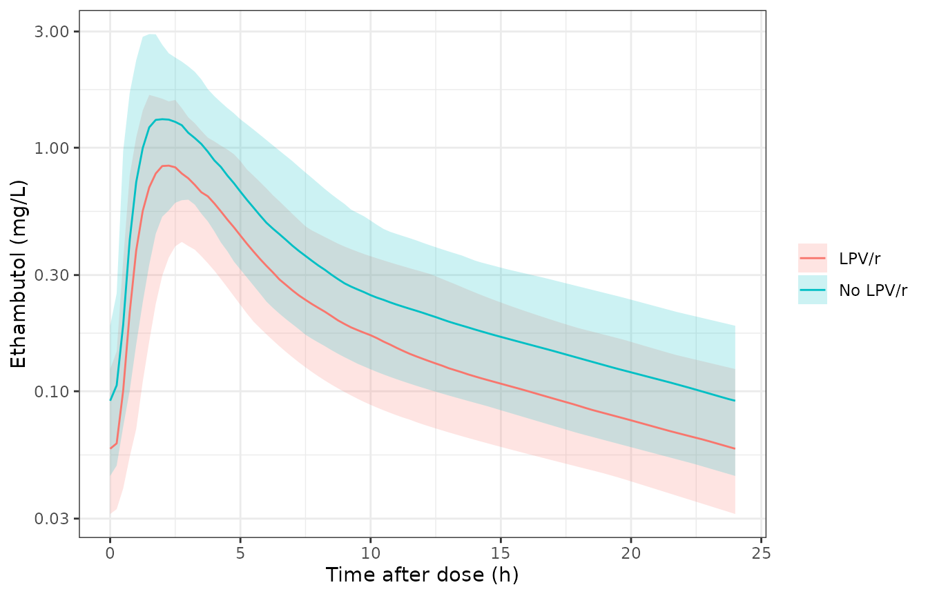

Simulated steady-state ethambutol plasma concentrations (median and 5th-95th percentiles of individual predictions), at 20.2 mg/kg ethambutol dihydrochloride once daily, by lopinavir/ritonavir co-treatment. Compare with the Figure 1 VPC of Tikiso 2022 stratified by HIV treatment.

PKNCA validation

conc <- ss |>
  dplyr::filter(!is.na(Cc)) |>
  dplyr::select(id, arm, tad, Cc)
dose <- cohort |>
  dplyr::transmute(id, arm, tad = 0, amt)

conc_obj <- PKNCA::PKNCAconc(conc, Cc ~ tad | arm + id)
dose_obj <- PKNCA::PKNCAdose(dose, amt ~ tad | arm + id)
intervals <- data.frame(
  start = 0, end = 24, cmax = TRUE, tmax = TRUE, auclast = TRUE
)
nca <- PKNCA::pk.nca(PKNCA::PKNCAdata(conc_obj, dose_obj, intervals = intervals))
nca_res <- as.data.frame(nca$result)

The paper’s Discussion reports the model-predicted steady-state ethambutol Cmax for the study children at the median 20.2 mg/kg dose: 1.66 mg/L (IQR 1.21-2.15) at 2.74 h without lopinavir/ritonavir and 0.882 mg/L (0.669-1.28) at 3.0 h with it.

published <- data.frame(
  arm = c("No LPV/r", "LPV/r"),
  cmax = c(1.66, 0.882),
  tmax = c(2.74, 3.0)
)
cmp <- nlmixr2lib::ncaComparisonTable(
  simulated = dplyr::filter(nca_res, PPTESTCD %in% c("cmax", "tmax")),
  reference = published,
  by = "arm",
  units = c(cmax = "mg/L", tmax = "h"),
  tolerance_pct = 20
)
cmp |>
  dplyr::rename("Arm" = arm) |>
  knitr::kable(caption = "Simulated vs published median steady-state Cmax and Tmax.")

Simulated vs published median steady-state Cmax and Tmax.

NCA parameter	Arm	Reference	Simulated	% diff
Cmax (mg/L)	No LPV/r	1.66	1.5	-9.6%
Cmax (mg/L)	LPV/r	0.882	0.928	+5.2%
Tmax (h)	No LPV/r	2.74	2	-27.0%*
Tmax (h)	LPV/r	3	2.25	-25.0%*

auc_summary <- nca_res |>
  dplyr::filter(PPTESTCD %in% c("cmax", "auclast")) |>
  dplyr::group_by(arm, PPTESTCD) |>
  dplyr::summarise(
    value = sprintf(
      "%.2f (%.2f-%.2f)", median(PPORRES), quantile(PPORRES, 0.25),
      quantile(PPORRES, 0.75)
    ),
    .groups = "drop"
  ) |>
  tidyr::pivot_wider(names_from = PPTESTCD, values_from = value)
auc_summary |>
  dplyr::rename(
    "Arm" = arm, "Cmax (mg/L)" = cmax, "AUC0-24 (mg*h/L)" = auclast
  ) |>
  knitr::kable(caption = "Simulated steady-state exposure, median (IQR).")

Simulated steady-state exposure, median (IQR).

Arm	AUC0-24 (mg*h/L)	Cmax (mg/L)
LPV/r	5.67 (4.55-7.19)	0.93 (0.68-1.14)
No LPV/r	8.69 (6.97-11.33)	1.50 (1.13-1.90)

Median Cmax reproduces the published values in both arms. Median Tmax is about 0.7 h earlier than published in both arms (flagged rows). The shift is the same in both arms, so it does not come from the lopinavir/ritonavir or the study effects. The typical DATiC child’s Tmax is about 1.8 h from the Table 2 ka (1.43 1/h) and MTT (40.4 min). Tmax rises with both quantities, so a median of 2.74 h would need a typical absorption roughly twice as slow as Table 2 reports. The published Tmax values are post hoc predictions for the actual children, whose individual absorption estimates (between-occasion variability of 63.7% on ka and 48.5% on MTT, crushed tablets in the youngest) need not centre on the typical values. The rate constants are kept exactly as published.

med_cmax <- nca_res |>
  dplyr::filter(PPTESTCD == "cmax") |>
  dplyr::group_by(arm) |>
  dplyr::summarise(med = median(PPORRES), .groups = "drop")
med_no <- med_cmax$med[med_cmax$arm == "No LPV/r"]
med_lpv <- med_cmax$med[med_cmax$arm == "LPV/r"]
stopifnot(
  # Centre of the distribution: a mis-transcribed clearance, volume, dose
  # conversion or absorption parameter moves the median by tens of percent.
  abs(med_no / 1.66 - 1) < 0.25,
  abs(med_lpv / 0.882 - 1) < 0.25,
  # The co-treatment contrast: published 0.882 / 1.66 = 0.53.
  abs((med_lpv / med_no) / (0.882 / 1.66) - 1) < 0.25
)
c(no_lpv = med_no, lpv = med_lpv, ratio = med_lpv / med_no)
#>    no_lpv       lpv     ratio 
#> 1.5008785 0.9279231 0.6182533

Weight-band dosing (Figures 2 and 3)

The paper simulated exposures by WHO weight band with the WHO-recommended doses and with its proposed optimised doses (Table 3, mg of ethambutol dihydrochloride), and compared Cmax with 2-6 mg/L and AUC0-24 with 16-29 mg*h/L. Here 25 children per weight band (200 per arm) are drawn uniformly within each band, with age obtained by inverting the scaled WHO weight-for-age curve; study is set to the DATiC reference.

bands <- data.frame(
  band = c("3-3.9", "4-5.9", "6-7.9", "8-11.9", "12-14.9", "15-19.9",
           "20-24.9", "25-35.9"),
  lo = c(3, 4, 6, 8, 12, 15, 20, 25),
  hi = c(3.9, 5.9, 7.9, 11.9, 14.9, 19.9, 24.9, 35.9),
  who = c(75, 100, 150, 200, 300, 400, 400, 600),
  opt_no_lpv = c(200, 300, 400, 600, 800, 800, 800, 1200),
  opt_lpv = c(300, 500, 800, 800, 1200, 1600, 1600, 1600)
)
band_kids <- bands |>
  dplyr::rowwise() |>
  dplyr::reframe(band = band, WT = stats::runif(25, lo, hi)) |>
  dplyr::mutate(
    AGE = pmax(stats::approx(who$wt * wt_factor, who$age, WT, rule = 2)$y, 0.05),
    HT = stats::approx(who$age, who$ht, AGE)$y * ht_factor,
    SEXF = stats::rbinom(dplyr::n(), 1, 0.55),
    GA = 39, STUDY_DNDI_SHINE = 0, OCC = 2
  ) |>
  dplyr::left_join(bands, by = "band")

band_cohort <- dplyr::bind_rows(
  dplyr::mutate(band_kids, CONMED_LOPINAVIR = 0, arm = "No LPV/r",
                regimen = "WHO", salt_mg = who),
  dplyr::mutate(band_kids, CONMED_LOPINAVIR = 1, arm = "LPV/r",
                regimen = "WHO", salt_mg = who),
  dplyr::mutate(band_kids, CONMED_LOPINAVIR = 0, arm = "No LPV/r",
                regimen = "Optimised", salt_mg = opt_no_lpv),
  dplyr::mutate(band_kids, CONMED_LOPINAVIR = 1, arm = "LPV/r",
                regimen = "Optimised", salt_mg = opt_lpv)
) |>
  dplyr::mutate(id = dplyr::row_number(), amt = salt_mg * 0.737)

band_ev <- ss_events(
  dplyr::select(band_cohort, id, amt, WT, HT, AGE, SEXF, GA,
                STUDY_DNDI_SHINE, OCC, CONMED_LOPINAVIR),
  obs_step = 0.25
)
band_sim <- rxode2::rxSolve(mod, band_ev, returnType = "data.frame") |>
  dplyr::filter(time >= 168)
stopifnot(!anyNA(band_sim$Cc))

band_exp <- band_sim |>
  dplyr::group_by(id) |>
  dplyr::summarise(
    cmax = max(Cc), auc = trap(time, Cc), .groups = "drop"
  ) |>
  dplyr::left_join(dplyr::select(band_cohort, id, band, arm, regimen), by = "id") |>
  dplyr::mutate(
    band = factor(band, levels = bands$band),
    regimen = factor(regimen, levels = c("WHO", "Optimised"))
  )

ggplot(band_exp, aes(band, cmax, fill = arm)) +
  annotate("rect", xmin = -Inf, xmax = Inf, ymin = 2, ymax = 6,
           alpha = 0.2, fill = "orange") +
  geom_boxplot(outlier.size = 0.5) +
  facet_wrap(~regimen) +
  labs(x = "Weight band (kg)", y = "Cmax (mg/L)", fill = NULL) +
  theme_bw() +
  theme(axis.text.x = element_text(angle = 45, hjust = 1))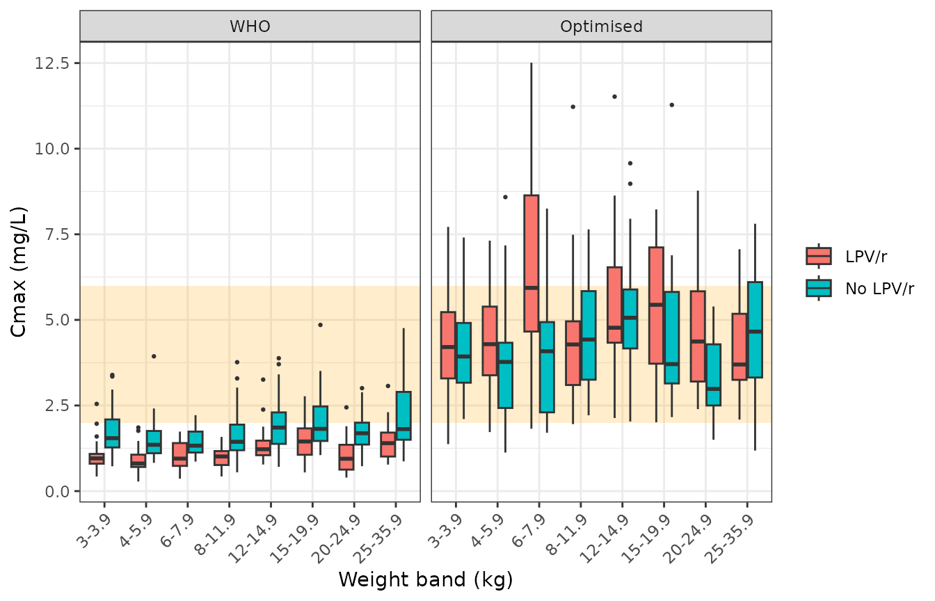

Simulated steady-state ethambutol Cmax by weight band with WHO-recommended (left) and optimised (right) dosing; shaded band 2-6 mg/L. Replicates Figure 2 of Tikiso 2022.

ggplot(band_exp, aes(band, auc, fill = arm)) +
  annotate("rect", xmin = -Inf, xmax = Inf, ymin = 16, ymax = 29,
           alpha = 0.2, fill = "orange") +
  geom_boxplot(outlier.size = 0.5) +
  facet_wrap(~regimen) +
  labs(x = "Weight band (kg)", y = "AUC0-24 (mg*h/L)", fill = NULL) +
  theme_bw() +
  theme(axis.text.x = element_text(angle = 45, hjust = 1))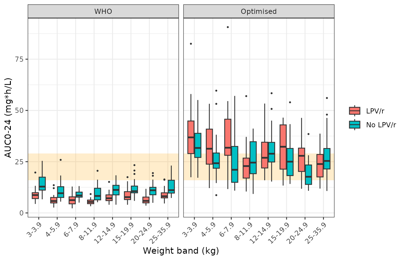

Simulated steady-state ethambutol AUC0-24 by weight band with WHO-recommended (left) and optimised (right) dosing; shaded band 16-29 mg*h/L. Replicates Figure 3 of Tikiso 2022.

The paper concludes that WHO doses leave most children below the adult Cmax and AUC ranges, and that roughly doubled (no LPV/r) or tripled (LPV/r) doses bring the typical child into them.

band_med <- band_exp |>
  dplyr::group_by(regimen, arm) |>
  dplyr::summarise(
    cmax = median(cmax), auc = median(auc), .groups = "drop"
  )
knitr::kable(
  dplyr::rename(band_med, "Regimen" = regimen, "Arm" = arm,
                "Median Cmax (mg/L)" = cmax, "Median AUC0-24 (mg*h/L)" = auc),
  digits = 2,
  caption = "Median simulated steady-state exposure across all weight bands."
)

Median simulated steady-state exposure across all weight bands.

Regimen	Arm	Median Cmax (mg/L)	Median AUC0-24 (mg*h/L)
WHO	LPV/r	1.06	6.97
WHO	No LPV/r	1.63	10.28
Optimised	LPV/r	4.63	28.35
Optimised	No LPV/r	4.06	25.14

who_med <- dplyr::filter(band_med, regimen == "WHO")
opt_med <- dplyr::filter(band_med, regimen == "Optimised")
stopifnot(
  all(who_med$cmax < 2),
  all(who_med$auc < 16),
  all(opt_med$cmax > 2 & opt_med$cmax < 6),
  all(opt_med$auc > 16 & opt_med$auc < 29)
)

Assumptions and deviations

• Dose basis. Every disposition parameter is apparent and relative to the dose expressed as ethambutol base (dihydrochloride x 0.737). The paper notes that comparing them with reports that dosed the salt requires multiplying by 1.357.
• Table 2 values, not control-stream initials. The supplementary control stream’s $THETA and $OMEGA are the starting values of the final run (for example CL 21.8 L/h on the salt-dose scale, i.e. about 16.1 L/h after the 0.737 conversion). Table 2 is used for every value.
• Variability scale. Table 2 percentages are read as the log-scale omega (omega^2 = (CV/100)^2): the control-stream initials for BOV on ka (0.403) and MTT (0.233) reproduce the tabulated 63.7% and 48.5% as sqrt(omega^2) (63.5%, 48.3%), not as sqrt(exp(omega^2) - 1) (70.4%, 51.0%).
• Inflated BOV on F for the unobserved dose is encoded by fixing the occasion-1 variance to 1.37^2 * 0.331^2, an exact re-expression of the control stream’s scaling of the occasion-1 deviate. The simulations above use occasion 2 (the observed dose) throughout.
• Between-occasion etas are not mu-referenced. rxode2 has no NONMEM-style occasion level, so the two-occasion BOV is expanded into indicator-selected etas and rxode2 warns that these etas are not mu-referenced. This only affects estimation speed-ups, not simulation.
• Explicit transit input. The Savic transit density is written out with podo() / tad() exactly as in the control stream $DES, instead of rxode2’s transit() built-in, which yields a zero input when combined with f(depot) <- 0. Each dose restarts the transit input; with MTT about 0.7 h against a 24 h interval no dose is lost, as the mass-balance check confirms.
• FFM is computed inside the model from WT, HT, AGE and SEXF with the control stream’s paediatric equation, so these four columns are needed even though only FFM enters the allometry. The reference FFM is the 7.7 kg cohort median (TVFFM), which Table 2 footnote b describes as a 10 kg child.
• Clearance maturation is not normalised: Table 2 CL is the fully mature value, so a 4-year-old has 99.6% of it. PMA50 is coded in months (Table 2); postmenstrual age is (AGE + GA/52) * 12 months.
• Censoring-specific error inflation (extra additive error for imputed BLQ records, near-infinite error for trailing BLQ records) belongs to the estimation dataset and is not part of the simulation model.
• Virtual cohort. Growth curves are approximate WHO medians scaled to the cohort’s undernutrition (factors 0.83 for weight and 0.95 for height), ages are log-normal by study, gestational age is 39 weeks, and every child receives exactly 20.2 mg/kg rather than a weight-band dose. The published Cmax values are post hoc predictions for the actual children, so the comparison checks the centre of the distribution rather than its tails.
• Weight-band simulations use the DATiC reference for the study effect (the paper does not state which study its simulations assumed) and 25 children per band instead of the paper’s more than 50,000.