Micafungin against Candida parapsilosis in vitro (Beredaki 2024)
Source:vignettes/articles/Beredaki_2024_micafungin.Rmd
Beredaki_2024_micafungin.RmdModel and source
Beredaki 2024 used an in vitro dialysis/diffusion pharmacokinetic/pharmacodynamic model to study micafungin against Candida parapsilosis. Conventional PK/PD targets (stasis, 50% of maximal effect) give a low probability of target attainment (PTA) for isolates the clinical breakpoint calls susceptible, even though echinocandins work well clinically against this species. The paper proposes a new target, the exposure giving 10% of the maximal effect at a low starting inoculum (EI10 = 28 tAUC0-24/MIC), which restores PTA >= 95% for susceptible isolates at the standard 100 mg daily dose.
The paper fitted four independent exposure-response curves – two media (RPMI with and without 10% pooled human serum) by two starting inocula (10^4 and 10^3 CFU/mL) – so the extraction is four model files sharing this vignette:
- 10% serum, 10^4 CFU/mL:
Beredaki_2024_micafungin_serum_inoc1e4 - 10% serum, 10^3 CFU/mL:
Beredaki_2024_micafungin_serum_inoc1e3 - serum-free RPMI, 10^4 CFU/mL:
Beredaki_2024_micafungin_rpmi_inoc1e4 - serum-free RPMI, 10^3 CFU/mL:
Beredaki_2024_micafungin_rpmi_inoc1e3 - Article: https://doi.org/10.1093/jac/dkad360
model_names <- c(
  serum_1e4 = "Beredaki_2024_micafungin_serum_inoc1e4",
  serum_1e3 = "Beredaki_2024_micafungin_serum_inoc1e3",
  rpmi_1e4 = "Beredaki_2024_micafungin_rpmi_inoc1e4",
  rpmi_1e3 = "Beredaki_2024_micafungin_rpmi_inoc1e3"
)
mods <- lapply(model_names, function(nm) rxode2::rxode(readModelDb(nm)))
# Named population-parameter vectors, used to evaluate the exposure-response
# curves directly from each model's ini().
thetas <- lapply(mods, function(m) m$theta)
Citation: Beredaki MI, Pournaras S, Meletiadis J. (2024). A new PK/PD target for assessing efficacy of micafungin against Candida parapsilosis. Journal of Antimicrobial Chemotherapy 79(1):157-165. doi:10.1093/jac/dkad360.
Description (10% serum, 10^3 CFU/mL): In vitro (Candida parapsilosis sensu stricto clinical isolates in RPMI-1640 with 10% pooled human serum, starting inoculum 10^3 CFU/mL; two-compartment closed dialysis/diffusion PK/PD model). Micafungin in vitro PK/PD model for the low inoculum that yields the paper’s proposed new PK/PD target (EI10 = 28 tAUC0-24/MIC). Micafungin was added once daily to the 10 mL internal compartment at a target total peak (tCmax 2-64 mg/L) and decayed mono-exponentially with the achieved in vitro half-life of 11 h. The 72 h change in log10 CFU/mL from the starting inoculum was related to the PK/PD index tAUC0-24/MIC by the sigmoidal variable-slope Emax model E = (Emax - Emin) * EI^n / (EI^n + EI50^n) + Emin, with Emax constrained to -2 log10 CFU/mL for this inoculum (Methods, ‘PK/PD analysis’); Emin = 5.23 and EI50 = 124 tAUC0-24/MIC are the published coefficients. The Hill coefficient is 1.45: the Results print n = -1.15, but that value contradicts both the paper’s own Table 1 targets (stasis 240, EI10 28, EI5 16 tAUC0-24/MIC, each reproduced by n = 1.45 to within 3%) and the curve drawn in Figure 4 (digitised n = 1.48), so the printed value is treated as a typesetting error for -1.45. The fungal density bact (CFU/mL) is integrated as d/dt(bact) = ln(10) * (change72 / 72) * bact so log10(bact) moves by exactly the fitted 72 h change. Companion files: Beredaki_2024_micafungin_serum_inoc1e4 (10^4 CFU/mL with serum) and Beredaki_2024_micafungin_rpmi_inoc1e4 / _rpmi_inoc1e3 (no serum).
Population
Three echinocandin-susceptible C. parapsilosis sensu stricto clinical isolates were tested – CP639, CP795 and CP732, with identical EUCAST and CLSI micafungin MICs of 2, 1 and 0.5 mg/L – together with a pan-echinocandin-resistant isolate (fks1 F652S plus the natural P660A polymorphism, MIC > 8 mg/L) against which no effect was seen at any exposure. In 10% human serum CP732 did not grow, so the serum curves rest on CP639 and CP795.
The dynamic model is an external compartment (a conical flask on a peristaltic pump) connected to an internal compartment: a 10 mL semipermeable cellulose dialysis tube (300 kDa cut-off) inoculated at 10^4 or 10^3 CFU/mL. The medium was RPMI 1640 buffered with MOPS to pH 7.0, with or without 10% heat-inactivated pooled human serum. Micafungin was added once daily for 72 h at free peak concentrations of 0.5, 1.8 and 4 mg/L in RPMI (Figure 2) and total peak concentrations of 2, 8, 32 and 64 mg/L with serum (Figure 3). The fungal load was sampled at 0, 4, 8, 24, 48 and 72 h (limit of detection 10 CFU/mL).
The same information is available programmatically via each model’s
population metadata, e.g.
readModelDb("Beredaki_2024_micafungin_serum_inoc1e3")()$population.
Source trace
The per-parameter origin is recorded as an in-file comment next to
each ini() entry. The table below collects them in one
place.
| Equation / parameter | Value | Source location |
|---|---|---|
d/dt(central) <- -kel * central;
Cc <- central / vc
|
n/a | Methods, “In vitro PK”: drug added at the target Cmax once daily, mono-exponential decay with a target half-life; Figure 1 |
lkel (serum) |
log(log(2) / 11) |
Results, “In vitro PK”: achieved t1/2 11 (7-18) h in RPMI + 10% serum |
lkel (RPMI) |
log(log(2) / 8) |
Results, “In vitro PK”: achieved t1/2 8 (6-11) h in RPMI |
lvc |
log(0.010) (fixed) |
Methods, “In vitro PK/PD model”: 10 mL internal compartment |
tau |
24 h (fixed) | Methods: drug added once daily; the index is AUC0-24/MIC |
cmax |
32 mg/L (serum) / 1.8 mg/L (RPMI) (fixed, design) | Figure 3 legend (tCmax 2, 8, 32, 64 mg/L) / Figure 2 legend (fCmax 0.5, 1.8, 4 mg/L) |
change72 <- e0 - (e0 - emax) * ei^hill / (ei^hill + ec50^hill) |
n/a | Methods, “PK/PD analysis”:
E = (Emax - Emin) * EI^n / (EI^n + EI50^n) + Emin
|
e0 (Emin) |
4 / 5.23 (serum 10^4 / 10^3) | Results, “PK/PD analysis”: “the Emin (4 versus 5.23)” |
e0 (Emin) |
3.78 / 4.40 (RPMI 10^4 / 10^3) | digitised from Figure 4, right panel |
emax |
-3 / -2 (10^4 / 10^3) (fixed) | Methods, “PK/PD analysis”: Emax constrained to -3 (10^4) and -2 (10^3) log10 CFU/mL |
lec50 (EI50) |
log(240) / log(124) tAUC0-24/MIC (serum
10^4 / 10^3) |
Table 1 and Results, “PK/PD analysis” |
lec50 (EI50) |
log(25.1) / log(41.3) fAUC0-24/MIC (RPMI
10^4 / 10^3) |
digitised from Figure 4, right panel (Table 1: 27 / 46) |
lhill (n) |
log(2.9) (serum 10^4) |
Results, “PK/PD analysis”: n = -2.9 (falling-curve sign convention) |
lhill (n) |
log(1.45) (serum 10^3) |
Table 1 targets and Figure 4; Results print -1.15 – see Assumptions and deviations |
lhill (n) |
log(2.56) / log(4.82) (RPMI 10^4 /
10^3) |
digitised from Figure 4, right panel |
mic |
2 mg/L (fixed) | Methods, “Candida isolates”: CP639 EUCAST/CLSI MIC 2 mg/L |
log10_cfu0 |
4.28 / 3.2 (serum), 3.94 / 3.06 (RPMI) (fixed) | Results, “In vitro PD”: measured mean t = 0 densities of the drug-free controls |
d/dt(bact) <- log(10) * (change72 / 72) * bact |
n/a | Methods, “In vitro PD”: effect assessed as the log10 CFU/mL change at 72 h vs the start of therapy |
propSd, addSd_log10cfu
|
0 (fixed) | Not reported; only R^2 (>= 0.90 with serum, >= 0.77 without) |
Reference PK/PD targets (Beredaki 2024 Table 1, mean with 95% CI). The serum curves are indexed on total AUC (tAUC0-24/MIC); the serum-free curves on the AUC in protein-free medium, i.e. fAUC0-24/MIC. The paper converts between the two with 99.75% protein binding (fAUC = 0.0025 x tAUC).
| Medium | Inoculum | Index | Stasis | EI50 | EI10 | EI5 |
|---|---|---|---|---|---|---|
| RPMI | 10^4 | fAUC/MIC | 28 (19-46) | 27 (18-39) | 10 (5-24) | 9 (3-21) |
| RPMI | 10^3 | fAUC/MIC | 50 (42-65) | 46 (38-56) | 27 (18-41) | 22 (13-39) |
| RPMI + 10% serum | 10^4 | tAUC/MIC | 272 (198-380) | 240 (180-320) | 113 (48-260) | 87 (30-249) |
| RPMI + 10% serum | 10^3 | tAUC/MIC | 240 (176-352) | 124 (88-184) | 28 (16-64) | 16 (8-48) |
Virtual cohort
The in vitro experiment has no virtual population: each arm is one
dialysis tube with a defined isolate (fixing mic) and a
defined target peak concentration (fixing cmax). Arms are
enumerated deterministically and every simulation below is a
typical-value solve; the models carry no between-subject variability,
matching a paper that reports none.
# Beredaki 2024 re-spiked the internal compartment to the target peak once daily
# (Figure 1: the target peaks are identical at 0, 24 and 48 h). The first dose
# raises the empty compartment to `cmax`; each later dose tops up the fraction
# lost over the preceding interval.
make_events <- function(cmax, kel, vc = 0.010, tau = 24, tmax = 72, dt = 0.25) {
  first_amt <- cmax * vc
  topup_amt <- cmax * (1 - exp(-kel * tau)) * vc
  dose_times <- seq(0, tmax - tau, by = tau)
  doses <- data.frame(
    time = dose_times,
    amt = c(first_amt, rep(topup_amt, length(dose_times) - 1L)),
    cmt = "central", evid = 1L, dvid = NA_integer_
  )
  # Observation rows sit on the ODE state `central`; `dvid = 1L` selects the Cc
  # endpoint. rxode2 returns every algebraic observable (Cc, ei, change72,
  # log10cfu) as a column at these rows.
  obs <- data.frame(
    time = seq(0, tmax, by = dt),
    amt = NA_real_, cmt = "central", evid = 0L, dvid = 1L
  )
  dplyr::bind_rows(doses, obs) |> dplyr::arrange(time, dplyr::desc(evid))
}

# One deterministic arm. `kel` defaults to the model's own achieved half-life.
solve_arm <- function(mod, cmax, mic = 2, kel = NULL, ...) {
  if (is.null(kel)) kel <- exp(mod$theta[["lkel"]])
  ev <- make_events(cmax = cmax, kel = kel, ...)
  rxode2::rxSolve(
    mod, ev,
    params = c(cmax = cmax, mic = mic, lkel = log(kel)),
    useLinCmt = FALSE, returnType = "data.frame"
  ) |>
    dplyr::mutate(cmax_nominal = cmax, mic_nominal = mic, thalf_nominal = log(2) / kel)
}
Replicate Figure 1: in vitro pharmacokinetics
Figure 1 (bottom panels) shows the measured q24h micafungin profiles
in the internal compartment against the target human profile (half-life
15 h), in RPMI (panel a) and in RPMI + 10% serum (panel b). The models
carry the achieved half-lives (8 h and 11 h); the target profiles are
obtained by overriding lkel.
pk_spec <- tibble::tribble(
  ~model,       ~panel,              ~cmax, ~label,
  "rpmi_1e4",   "(a) RPMI",            0.5, "fCmax 0.5 mg/L",
  "rpmi_1e4",   "(a) RPMI",            1.8, "fCmax 1.8 mg/L",
  "rpmi_1e4",   "(a) RPMI",            4.0, "fCmax 4 mg/L",
  "serum_1e4",  "(b) RPMI + 10% serum",  2, "tCmax 2 mg/L",
  "serum_1e4",  "(b) RPMI + 10% serum",  8, "tCmax 8 mg/L",
  "serum_1e4",  "(b) RPMI + 10% serum", 32, "tCmax 32 mg/L"
)

# Every arm at the achieved and at the target half-life, over `tmax` hours.
solve_pk_spec <- function(tmax) {
  dplyr::bind_rows(lapply(seq_len(nrow(pk_spec)), function(i) {
    s <- pk_spec[i, ]
    mod <- mods[[s$model]]
    dplyr::bind_rows(
      solve_arm(mod, cmax = s$cmax, tmax = tmax) |>
        dplyr::mutate(profile = "in vitro (achieved t1/2)"),
      solve_arm(mod, cmax = s$cmax, kel = log(2) / 15, tmax = tmax) |>
        dplyr::mutate(profile = "target (t1/2 15 h)")
    ) |>
      dplyr::mutate(panel = s$panel, label = s$label, arm = paste(s$label, "-", profile))
  }))
}

pk_arms <- solve_pk_spec(tmax = 72)

ggplot(pk_arms, aes(time, Cc, colour = label, linetype = profile)) +
  geom_line() +
  facet_wrap(~panel, scales = "free_y") +
  scale_x_continuous(breaks = seq(0, 72, by = 12)) +
  labs(
    x = "Time (h)", y = "Micafungin concentration (mg/L)",
    colour = NULL, linetype = NULL,
    title = "Figure 1 -- simulated q24h micafungin profiles in the internal compartment",
    caption = "Replicates Figure 1 (bottom panels) of Beredaki 2024."
  ) +
  theme(legend.position = "bottom", legend.text = element_text(size = 7))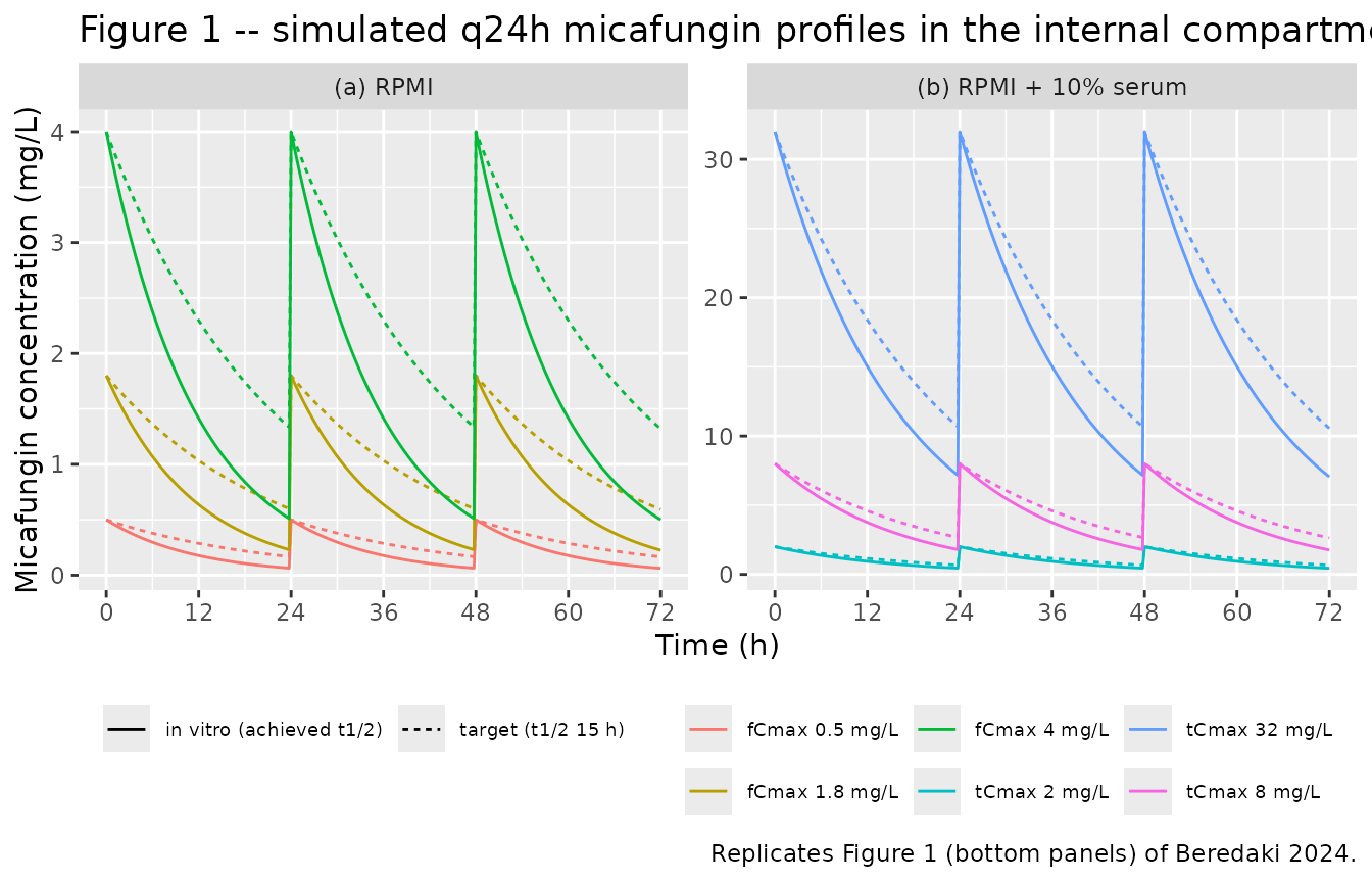
PKNCA validation
Non-compartmental analysis over the first dosing interval – the window that defines the paper’s PK/PD index. Because the compartment is re-spiked at 24 h, the 24 h observation of the multiple-dose profile above is the new peak, not the trough; the NCA therefore uses a separate solve that stops at 24 h, which is identical to the first interval of the q24h regimen. The arm is the treatment grouping variable.
pk_first <- solve_pk_spec(tmax = 24)

sim_nca <- pk_first |>
  dplyr::filter(!is.na(Cc)) |>
  dplyr::mutate(id = 1L) |>
  dplyr::select(id, time, Cc, arm)

# Guarantee a time = 0 record per arm. The dose is a bolus spike, so the t = 0
# value is already the peak; the bind_rows/distinct pattern is a defensive no-op.
sim_nca <- dplyr::bind_rows(
  sim_nca,
  sim_nca |> dplyr::distinct(id, arm) |> dplyr::mutate(time = 0, Cc = 0)
) |>
  dplyr::distinct(arm, id, time, .keep_all = TRUE) |>
  dplyr::arrange(arm, id, time)

conc_obj <- PKNCA::PKNCAconc(sim_nca, Cc ~ time | arm + id)

dose_df <- pk_first |>
  dplyr::distinct(arm, cmax_nominal) |>
  dplyr::mutate(id = 1L, time = 0, amt = cmax_nominal * 0.010) |>
  dplyr::select(id, time, amt, arm)

dose_obj <- PKNCA::PKNCAdose(dose_df, amt ~ time | arm + id)

intervals <- data.frame(
  start = 0, end = 24,
  cmax = TRUE, tmax = TRUE, auclast = TRUE, half.life = TRUE
)

nca_res <- PKNCA::pk.nca(PKNCA::PKNCAdata(conc_obj, dose_obj, intervals = intervals))

nca_tidy <- as.data.frame(nca_res) |>
  dplyr::filter(PPTESTCD %in% c("cmax", "tmax", "auclast", "half.life")) |>
  dplyr::select(arm, PPTESTCD, PPORRES) |>
  tidyr::pivot_wider(names_from = PPTESTCD, values_from = PPORRES)

nca_tidy |>
  dplyr::mutate(dplyr::across(where(is.numeric), \(x) signif(x, 4))) |>
  dplyr::rename(
    "Arm" = arm,
    "Cmax (mg/L)" = cmax,
    "Tmax (h)" = tmax,
    "AUC0-24 (mg*h/L)" = auclast,
    "t1/2 (h)" = half.life
  ) |>
knitr::kable(caption = "PKNCA results for the simulated in vitro PK arms.")| Arm | AUC0-24 (mg*h/L) | Cmax (mg/L) | Tmax (h) | t1/2 (h) |
|---|---|---|---|---|
| fCmax 0.5 mg/L - in vitro (achieved t1/2) | 5.049 | 0.5 | 0 | 8 |
| fCmax 0.5 mg/L - target (t1/2 15 h) | 7.251 | 0.5 | 0 | 15 |
| fCmax 1.8 mg/L - in vitro (achieved t1/2) | 18.180 | 1.8 | 0 | 8 |
| fCmax 1.8 mg/L - target (t1/2 15 h) | 26.100 | 1.8 | 0 | 15 |
| fCmax 4 mg/L - in vitro (achieved t1/2) | 40.400 | 4.0 | 0 | 8 |
| fCmax 4 mg/L - target (t1/2 15 h) | 58.010 | 4.0 | 0 | 15 |
| tCmax 2 mg/L - in vitro (achieved t1/2) | 24.740 | 2.0 | 0 | 11 |
| tCmax 2 mg/L - target (t1/2 15 h) | 29.000 | 2.0 | 0 | 15 |
| tCmax 32 mg/L - in vitro (achieved t1/2) | 395.900 | 32.0 | 0 | 11 |
| tCmax 32 mg/L - target (t1/2 15 h) | 464.100 | 32.0 | 0 | 15 |
| tCmax 8 mg/L - in vitro (achieved t1/2) | 98.980 | 8.0 | 0 | 11 |
| tCmax 8 mg/L - target (t1/2 15 h) | 116.000 | 8.0 | 0 | 15 |
Comparison against published PK values
Beredaki 2024 specifies the target peak of every arm and reports the achieved in vitro half-lives (8 h in RPMI, 11 h with serum) and the target human half-life (15 h).
published_pk <- pk_first |>
  dplyr::distinct(arm, cmax = cmax_nominal, half.life = thalf_nominal)

cmp_pk <- nlmixr2lib::ncaComparisonTable(
  simulated = nca_tidy,
  reference = published_pk,
  by = "arm",
  params = c("cmax", "half.life"),
  units = c(cmax = "mg/L", half.life = "h"),
  tolerance_pct = 20
)

knitr::kable(
  cmp_pk,
  caption = paste(
    "Simulated vs published in vitro PK. Reference Cmax values are the target",
    "peak concentrations (Figures 1-3); reference half-lives are the achieved",
    "values from Results (8 h RPMI, 11 h serum) or the 15 h design target.",
    "* differs from reference by >20%."
  )
)| NCA parameter | arm | Reference | Simulated | % diff |
|---|---|---|---|---|
| Cmax (mg/L) | fCmax 0.5 mg/L - in vitro (achieved t1/2) | 0.5 | 0.5 | -0.0% |
| Cmax (mg/L) | fCmax 0.5 mg/L - target (t1/2 15 h) | 0.5 | 0.5 | -0.0% |
| Cmax (mg/L) | fCmax 1.8 mg/L - in vitro (achieved t1/2) | 1.8 | 1.8 | -0.0% |
| Cmax (mg/L) | fCmax 1.8 mg/L - target (t1/2 15 h) | 1.8 | 1.8 | -0.0% |
| Cmax (mg/L) | fCmax 4 mg/L - in vitro (achieved t1/2) | 4 | 4 | -0.0% |
| Cmax (mg/L) | fCmax 4 mg/L - target (t1/2 15 h) | 4 | 4 | -0.0% |
| Cmax (mg/L) | tCmax 2 mg/L - in vitro (achieved t1/2) | 2 | 2 | -0.0% |
| Cmax (mg/L) | tCmax 2 mg/L - target (t1/2 15 h) | 2 | 2 | -0.0% |
| Cmax (mg/L) | tCmax 8 mg/L - in vitro (achieved t1/2) | 8 | 8 | -0.0% |
| Cmax (mg/L) | tCmax 8 mg/L - target (t1/2 15 h) | 8 | 8 | -0.0% |
| Cmax (mg/L) | tCmax 32 mg/L - in vitro (achieved t1/2) | 32 | 32 | -0.0% |
| Cmax (mg/L) | tCmax 32 mg/L - target (t1/2 15 h) | 32 | 32 | -0.0% |
| t½ (h) | fCmax 0.5 mg/L - in vitro (achieved t1/2) | 8 | 8 | +0.0% |
| t½ (h) | fCmax 0.5 mg/L - target (t1/2 15 h) | 15 | 15 | +0.0% |
| t½ (h) | fCmax 1.8 mg/L - in vitro (achieved t1/2) | 8 | 8 | +0.0% |
| t½ (h) | fCmax 1.8 mg/L - target (t1/2 15 h) | 15 | 15 | -0.0% |
| t½ (h) | fCmax 4 mg/L - in vitro (achieved t1/2) | 8 | 8 | -0.0% |
| t½ (h) | fCmax 4 mg/L - target (t1/2 15 h) | 15 | 15 | -0.0% |
| t½ (h) | tCmax 2 mg/L - in vitro (achieved t1/2) | 11 | 11 | +0.0% |
| t½ (h) | tCmax 2 mg/L - target (t1/2 15 h) | 15 | 15 | +0.0% |
| t½ (h) | tCmax 8 mg/L - in vitro (achieved t1/2) | 11 | 11 | +0.0% |
| t½ (h) | tCmax 8 mg/L - target (t1/2 15 h) | 15 | 15 | +0.0% |
| t½ (h) | tCmax 32 mg/L - in vitro (achieved t1/2) | 11 | 11 | -0.0% |
| t½ (h) | tCmax 32 mg/L - target (t1/2 15 h) | 15 | 15 | -0.0% |
The PK/PD index inside each model is the closed form of the
first-interval AUC, cmax * (1 - exp(-kel * tau)) / kel. It
must agree with the PKNCA AUC0-24 of the simulated profile – the
strictest check that dose amounts, volume and elimination are wired
together correctly.
chk <- nca_tidy |>
  dplyr::left_join(published_pk, by = "arm", suffix = c("_sim", "_ref")) |>
  dplyr::left_join(
    pk_first |>
      dplyr::filter(time == 0) |>
      dplyr::mutate(auc_closed = dplyr::coalesce(tauc24, fauc24)) |>
      dplyr::distinct(arm, auc_closed),
    by = "arm"
  )
# Same drawn parameters on both sides, so these are numerical-error bounds.
stopifnot(max(abs(chk$cmax_sim / chk$cmax_ref - 1)) < 0.01)
stopifnot(max(abs(chk$half.life_sim / chk$half.life_ref - 1)) < 0.01)
stopifnot(max(abs(chk$auclast / chk$auc_closed - 1)) < 0.01)
Replicate Figure 4: the exposure-response relationships
Figure 4 plots the 72 h change in log10 CFU/mL against fAUC0-24/MIC
with 10% serum (left, R^2 >= 0.90) and in RPMI (right, R^2 >=
0.77). The packaged models reproduce the curves directly from
e0, emax, ec50 and
hill; the serum curves are drawn on the fAUC axis with the
paper’s 99.75% protein binding.
fu <- 0.0025

# Exposure-response evaluated from a model's theta vector on the model's
# native index (tAUC/MIC for serum, fAUC/MIC for RPMI).
er_curve <- function(th, ei) {
  e0 <- th[["e0"]]
  emax <- th[["emax"]]
  ec50 <- exp(th[["lec50"]])
  hill <- exp(th[["lhill"]])
  e0 - (e0 - emax) * ei^hill / (ei^hill + ec50^hill)
}

curve_spec <- tibble::tribble(
  ~model,      ~panel,              ~inoculum,     ~to_fauc,
  "serum_1e4", "RPMI + 10% serum", "10^4 CFU/mL",  fu,
  "serum_1e3", "RPMI + 10% serum", "10^3 CFU/mL",  fu,
  "rpmi_1e4",  "RPMI",             "10^4 CFU/mL",  1,
  "rpmi_1e3",  "RPMI",             "10^3 CFU/mL",  1
)

fauc_grid <- 10^seq(-2, 2, length.out = 400)
curves <- dplyr::bind_rows(lapply(seq_len(nrow(curve_spec)), function(i) {
  s <- curve_spec[i, ]
  tibble::tibble(
    fauc_mic = fauc_grid,
    change = er_curve(thetas[[s$model]], fauc_grid / s$to_fauc),
    panel = s$panel, inoculum = s$inoculum
  )
}))

ggplot(curves, aes(fauc_mic, change, colour = inoculum)) +
  geom_hline(yintercept = 0, linetype = "dashed") +
  geom_line(linewidth = 0.8) +
  facet_wrap(~panel) +
  scale_x_log10() +
  scale_colour_manual(values = c("10^4 CFU/mL" = "black", "10^3 CFU/mL" = "grey60")) +
  labs(
    x = "micafungin fAUC0-24 / MIC", y = "72 h change in log10 CFU/mL",
    colour = "Starting inoculum",
    title = "Figure 4 -- in vitro exposure-response of micafungin",
    caption = "Replicates Figure 4 of Beredaki 2024. Dashed line = stasis."
  ) +
  theme(legend.position = "bottom")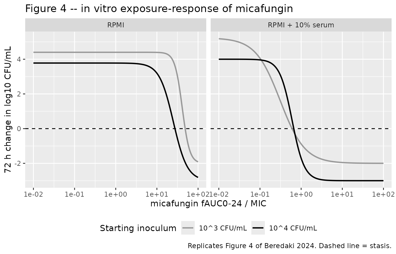
Validation against the Table 1 PK/PD targets
Each packaged curve is inverted to recover the exposure index at
stasis (no change from the starting inoculum) and at 50%, 10% and 5% of
the maximal effect, where “x% of the maximal effect” is the exposure
that moves the change x% of the way from e0 to
emax.
invert_curve <- function(th, target_change) {
  stats::uniroot(
    function(lei) er_curve(th, exp(lei)) - target_change,
    interval = log(c(1e-4, 1e6)), tol = 1e-10
  )$root |> exp()
}

target_change <- function(th, endpoint) {
  e0 <- th[["e0"]]
  emax <- th[["emax"]]
  switch(endpoint,
    stasis = 0,
    EI50 = e0 - 0.50 * (e0 - emax),
    EI10 = e0 - 0.10 * (e0 - emax),
    EI5 = e0 - 0.05 * (e0 - emax)
  )
}

table1 <- tibble::tribble(
  ~model,      ~index,      ~endpoint, ~reported, ~lo,   ~hi,
  "serum_1e4", "tAUC/MIC",  "stasis",  272,       198,   380,
  "serum_1e4", "tAUC/MIC",  "EI50",    240,       180,   320,
  "serum_1e4", "tAUC/MIC",  "EI10",    113,        48,   260,
  "serum_1e4", "tAUC/MIC",  "EI5",      87,        30,   249,
  "serum_1e3", "tAUC/MIC",  "stasis",  240,       176,   352,
  "serum_1e3", "tAUC/MIC",  "EI50",    124,        88,   184,
  "serum_1e3", "tAUC/MIC",  "EI10",     28,        16,    64,
  "serum_1e3", "tAUC/MIC",  "EI5",      16,         8,    48,
  "rpmi_1e4",  "fAUC/MIC",  "stasis",   28,        19,    46,
  "rpmi_1e4",  "fAUC/MIC",  "EI50",     27,        18,    39,
  "rpmi_1e4",  "fAUC/MIC",  "EI10",     10,         5,    24,
  "rpmi_1e4",  "fAUC/MIC",  "EI5",       9,         3,    21,
  "rpmi_1e3",  "fAUC/MIC",  "stasis",   50,        42,    65,
  "rpmi_1e3",  "fAUC/MIC",  "EI50",     46,        38,    56,
  "rpmi_1e3",  "fAUC/MIC",  "EI10",     27,        18,    41,
  "rpmi_1e3",  "fAUC/MIC",  "EI5",      22,        13,    39
) |>
  dplyr::rowwise() |>
  dplyr::mutate(
    simulated = invert_curve(thetas[[model]], target_change(thetas[[model]], endpoint))
  ) |>
  dplyr::ungroup() |>
  dplyr::mutate(pct_diff = 100 * (simulated / reported - 1))

table1 |>
  dplyr::mutate(
    simulated = signif(simulated, 3),
    pct_diff = round(pct_diff, 1),
    ci = paste0(lo, "-", hi)
  ) |>
  dplyr::select(model, index, endpoint, reported, ci, simulated, pct_diff) |>
  dplyr::rename(
    "Model" = model,
    "Index" = index,
    "Target" = endpoint,
    "Table 1" = reported,
    "Table 1 95% CI" = ci,
    "Packaged model" = simulated,
    "Difference (%)" = pct_diff
  ) |>
knitr::kable(caption = "Packaged exposure-response curves vs Beredaki 2024 Table 1.")| Model | Index | Target | Table 1 | Table 1 95% CI | Packaged model | Difference (%) |
|---|---|---|---|---|---|---|
| serum_1e4 | tAUC/MIC | stasis | 272 | 198-380 | 265.00 | -2.6 |
| serum_1e4 | tAUC/MIC | EI50 | 240 | 180-320 | 240.00 | 0.0 |
| serum_1e4 | tAUC/MIC | EI10 | 113 | 48-260 | 113.00 | -0.4 |
| serum_1e4 | tAUC/MIC | EI5 | 87 | 30-249 | 86.90 | -0.1 |
| serum_1e3 | tAUC/MIC | stasis | 240 | 176-352 | 241.00 | 0.3 |
| serum_1e3 | tAUC/MIC | EI50 | 124 | 88-184 | 124.00 | 0.0 |
| serum_1e3 | tAUC/MIC | EI10 | 28 | 16-64 | 27.20 | -2.7 |
| serum_1e3 | tAUC/MIC | EI5 | 16 | 8-48 | 16.30 | 1.7 |
| rpmi_1e4 | fAUC/MIC | stasis | 28 | 19-46 | 27.50 | -1.9 |
| rpmi_1e4 | fAUC/MIC | EI50 | 27 | 18-39 | 25.10 | -7.0 |
| rpmi_1e4 | fAUC/MIC | EI10 | 10 | 5-24 | 10.60 | 6.4 |
| rpmi_1e4 | fAUC/MIC | EI5 | 9 | 3-21 | 7.95 | -11.7 |
| rpmi_1e3 | fAUC/MIC | stasis | 50 | 42-65 | 48.60 | -2.7 |
| rpmi_1e3 | fAUC/MIC | EI50 | 46 | 38-56 | 41.30 | -10.2 |
| rpmi_1e3 | fAUC/MIC | EI10 | 27 | 18-41 | 26.20 | -3.0 |
| rpmi_1e3 | fAUC/MIC | EI5 | 22 | 13-39 | 22.40 | 1.9 |
# Every recovered target must fall inside the paper's own 95% CI.
stopifnot(all(table1$simulated > table1$lo & table1$simulated < table1$hi))
# The serum curves use the published coefficients: every target within 5%.
serum_rows <- table1$model %in% c("serum_1e4", "serum_1e3")
stopifnot(max(abs(table1$pct_diff[serum_rows])) < 5)
# The digitised serum-free curves: stasis, EI10 and EI5 within 15%; EI50 is
# where Table 1 and the drawn curve disagree (see Assumptions and deviations).
rpmi_rows <- !serum_rows & table1$endpoint != "EI50"
stopifnot(max(abs(table1$pct_diff[rpmi_rows])) < 15)
The two serum curves, built from the published coefficients, reproduce all eight Table 1 serum targets to within 3%. In particular the new target the paper proposes – EI10 at 10^3 CFU/mL – comes out at 27.2 tAUC0-24/MIC against the reported 28.
The printed Hill coefficient of the 10^3 CFU/mL serum curve
Results print n = -1.15 for the 10^3 CFU/mL serum curve. The table below shows what that value would give, holding the other published coefficients (Emin 5.23, Emax -2, EI50 124) fixed, against the packaged n = 1.45.
hill_check <- tibble::tibble(endpoint = c("stasis", "EI10", "EI5"), reported = c(240, 28, 16))
th_115 <- thetas$serum_1e3
th_115[["lhill"]] <- log(1.15)
hill_check$`n = 1.15 (as printed)` <- vapply(
  hill_check$endpoint,
  function(ep) invert_curve(th_115, target_change(th_115, ep)),
  numeric(1)
)
hill_check$`n = 1.45 (packaged)` <- vapply(
  hill_check$endpoint,
  function(ep) invert_curve(thetas$serum_1e3, target_change(thetas$serum_1e3, ep)),
  numeric(1)
)
hill_check |>
  dplyr::mutate(dplyr::across(where(is.numeric), \(x) signif(x, 3))) |>
  dplyr::rename("Target" = endpoint, "Table 1 (tAUC0-24/MIC)" = reported) |>
knitr::kable(caption = "Effect of the printed vs packaged Hill coefficient on the 10^3 CFU/mL serum targets.")| Target | Table 1 (tAUC0-24/MIC) | n = 1.15 (as printed) | n = 1.45 (packaged) |
|---|---|---|---|
| stasis | 240 | 286.00 | 241.0 |
| EI10 | 28 | 18.40 | 27.2 |
| EI5 | 16 | 9.58 | 16.3 |
Replicate Figures 2 and 3: time-kill curves
Figures 2 and 3 show the time-kill curves for each isolate and regimen in RPMI and with 10% serum. The packaged models spread the fitted 72 h change uniformly across the window, so each trajectory is a straight line on the log10 scale that lands on the fitted endpoint at 72 h; the curvature within 72 h is not modelled.
isolates <- tibble::tribble(
  ~isolate,          ~mic,
  "CP639 (MIC 2)",     2,
  "CP795 (MIC 1)",     1,
  "CP732 (MIC 0.5)", 0.5
)
regimens <- tibble::tribble(
  ~medium,   ~cmax,
  "rpmi",      0,
  "rpmi",      0.5,
  "rpmi",      1.8,
  "rpmi",      4,
  "serum",     0,
  "serum",     2,
  "serum",     8,
  "serum",    32,
  "serum",    64
)
inocula <- tibble::tibble(inoculum = c("1e4", "1e3"))

tk_grid <- tidyr::expand_grid(regimens, inocula, isolates) |>
  # CP732 did not grow in 10% serum, so it has no serum time-kill curve.
  dplyr::filter(!(medium == "serum" & mic == 0.5)) |>
  dplyr::mutate(model = paste0(medium, "_", inoculum))

timekill <- dplyr::bind_rows(lapply(seq_len(nrow(tk_grid)), function(i) {
  g <- tk_grid[i, ]
  solve_arm(mods[[g$model]], cmax = g$cmax, mic = g$mic, dt = 4) |>
    dplyr::select(time, log10cfu, ei, change72) |>
    dplyr::mutate(
      medium = g$medium, inoculum = g$inoculum, isolate = g$isolate, mic = g$mic,
      cmax = g$cmax,
      regimen = if (g$cmax == 0) {
        "drug-free control"
      } else {
        paste0(if (g$medium == "rpmi") "fCmax " else "tCmax ", g$cmax, " mg/L")
      }
    )
}))

timekill |>
  dplyr::filter(medium == "rpmi") |>
  ggplot(aes(time, log10cfu, colour = regimen)) +
  geom_line() +
  geom_hline(yintercept = 1, linetype = "dotted") +
  facet_grid(paste("inoculum", inoculum) ~ isolate) +
  scale_x_continuous(breaks = seq(0, 72, by = 24)) +
  labs(
    x = "Time (h)", y = "log10 CFU/mL", colour = NULL,
    title = "Figure 2 -- in vitro time-kill in RPMI",
    caption = "Replicates Figure 2 of Beredaki 2024. Dotted line = limit of detection."
  ) +
  theme(legend.position = "bottom")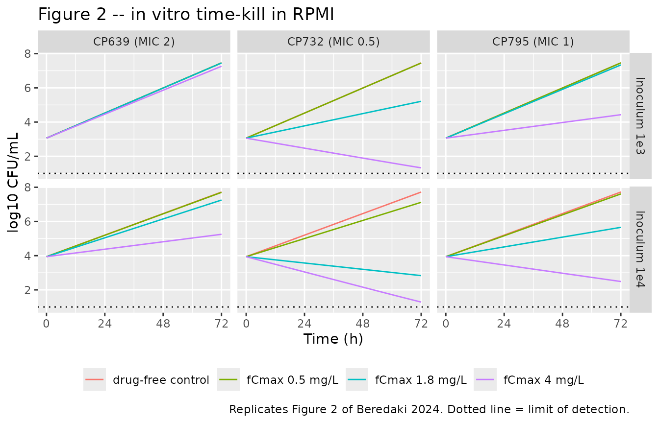
timekill |>
  dplyr::filter(medium == "serum") |>
  ggplot(aes(time, log10cfu, colour = regimen)) +
  geom_line() +
  geom_hline(yintercept = 1, linetype = "dotted") +
  facet_grid(paste("inoculum", inoculum) ~ isolate) +
  scale_x_continuous(breaks = seq(0, 72, by = 24)) +
  labs(
    x = "Time (h)", y = "log10 CFU/mL", colour = NULL,
    title = "Figure 3 -- in vitro time-kill in RPMI + 10% pooled human serum",
    caption = "Replicates Figure 3 of Beredaki 2024. Dotted line = limit of detection."
  ) +
  theme(legend.position = "bottom")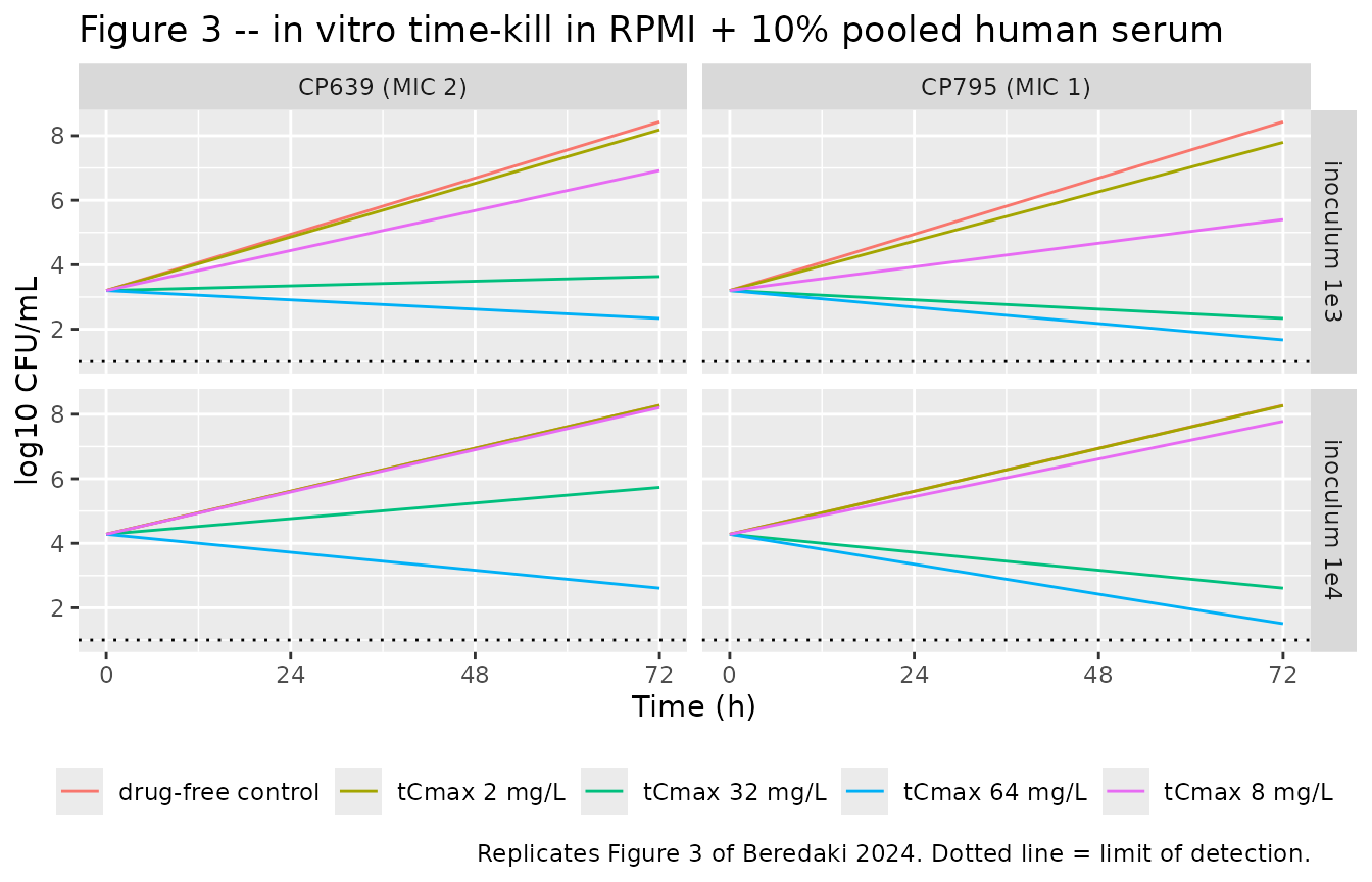
endpoints <- timekill |>
  dplyr::group_by(medium, inoculum, isolate, mic, cmax, regimen) |>
  dplyr::summarise(
    change_72h = dplyr::last(log10cfu) - dplyr::first(log10cfu),
    .groups = "drop"
  )

endpoints |>
  dplyr::mutate(change_72h = round(change_72h, 2)) |>
  dplyr::select(medium, inoculum, isolate, regimen, change_72h) |>
  tidyr::pivot_wider(names_from = isolate, values_from = change_72h) |>
  dplyr::rename("Medium" = medium, "Inoculum" = inoculum, "Regimen" = regimen) |>
knitr::kable(caption = "Model 72 h change in log10 CFU/mL by medium, inoculum, regimen and isolate.")| Medium | Inoculum | Regimen | CP639 (MIC 2) | CP732 (MIC 0.5) | CP795 (MIC 1) |
|---|---|---|---|---|---|
| rpmi | 1e3 | drug-free control | 4.40 | 4.40 | 4.40 |
| rpmi | 1e3 | fCmax 0.5 mg/L | 4.40 | 4.39 | 4.40 |
| rpmi | 1e3 | fCmax 1.8 mg/L | 4.40 | 2.15 | 4.28 |
| rpmi | 1e3 | fCmax 4 mg/L | 4.20 | -1.74 | 1.37 |
| rpmi | 1e4 | drug-free control | 3.78 | 3.78 | 3.78 |
| rpmi | 1e4 | fCmax 0.5 mg/L | 3.76 | 3.18 | 3.67 |
| rpmi | 1e4 | fCmax 1.8 mg/L | 3.31 | -1.11 | 1.72 |
| rpmi | 1e4 | fCmax 4 mg/L | 1.31 | -2.65 | -1.45 |
| serum | 1e3 | drug-free control | 5.23 | NA | 5.23 |
| serum | 1e3 | tCmax 2 mg/L | 4.98 | NA | 4.59 |
| serum | 1e3 | tCmax 8 mg/L | 3.72 | NA | 2.20 |
| serum | 1e3 | tCmax 32 mg/L | 0.43 | NA | -0.87 |
| serum | 1e3 | tCmax 64 mg/L | -0.87 | NA | -1.53 |
| serum | 1e4 | drug-free control | 4.00 | NA | 4.00 |
| serum | 1e4 | tCmax 2 mg/L | 4.00 | NA | 3.99 |
| serum | 1e4 | tCmax 8 mg/L | 3.93 | NA | 3.50 |
| serum | 1e4 | tCmax 32 mg/L | 1.45 | NA | -1.67 |
| serum | 1e4 | tCmax 64 mg/L | -1.67 | NA | -2.77 |
end_of <- function(med, ino, mic_val, cmax_val) {
  endpoints$change_72h[
    endpoints$medium == med & endpoints$inoculum == ino &
      endpoints$mic == mic_val & endpoints$cmax == cmax_val
  ]
}
# Results, "In RPMI": the initial log10 CFU/mL decreased for isolates with
# MIC <= 1 mg/L at fCmax 4 mg/L -- and not for CP639 (MIC 2). At 10^3 CFU/mL
# the CP795 arm (fAUC0-24/MIC about 40) lies below that curve's own stasis
# target of 50, so the fitted curve predicts growth there; see the text below.
stopifnot(end_of("rpmi", "1e4", 1, 4) < 0, end_of("rpmi", "1e4", 0.5, 4) < 0)
stopifnot(end_of("rpmi", "1e3", 0.5, 4) < 0)
stopifnot(end_of("rpmi", "1e4", 2, 4) > 0, end_of("rpmi", "1e3", 2, 4) > 0)
# Results, "In RPMI with 10% human serum": a fungicidal effect at tCmax 64 mg/L
# (2-2.8 log10 CFU/mL reduction) for both isolates at 10^4 CFU/mL.
stopifnot(end_of("serum", "1e4", 1, 64) < -2, end_of("serum", "1e4", 1, 64) > -2.8)
stopifnot(end_of("serum", "1e4", 2, 64) < -1.5)
# ... and a fungistatic effect at tCmax 32 mg/L against both isolates at
# 10^3 CFU/mL.
stopifnot(abs(end_of("serum", "1e3", 2, 32)) < 1, abs(end_of("serum", "1e3", 1, 32)) < 1)
# Drug-free controls reproduce each curve's zero-exposure change exactly.
ctrl <- endpoints |> dplyr::filter(cmax == 0)
ctrl_e0 <- vapply(paste0(ctrl$medium, "_", ctrl$inoculum), function(m) thetas[[m]][["e0"]], numeric(1))
stopifnot(max(abs(ctrl$change_72h - ctrl_e0)) < 1e-3)
The model reproduces most of the Results’ threshold statements: killing in RPMI at fCmax 4 mg/L for the MIC <= 1 mg/L isolates only (with one exception, below), a 2-2.8 log10 reduction for CP795 at tCmax 64 mg/L with serum (CP639 reaches -1.67, slightly short of the reported 2 log10), and stasis at tCmax 32 mg/L with serum at the low inoculum.
The exception is CP795 at fCmax 4 mg/L with the 10^3 CFU/mL inoculum. Figure 2 shows that arm falling from about 2.5 to the limit of detection, but its exposure under the reported 8 h half-life, an fAUC0-24/MIC of about 40.4, lies below the 10^3 CFU/mL curve’s own Table 1 stasis target of 50, so the published exposure-response predicts net growth (1.37 log10 CFU/mL). The fitted curve is steep there (n about 4.8), so a modest difference between the idealised and the measured AUC of that experiment moves the prediction across stasis.
Bridging to human data: probability of target attainment
Figure 5 carries the serum targets to patients by Monte Carlo simulation of 5000 patients given 100 mg micafungin IV q24h, whose total AUC0-24 is normal with mean 97 and SD 29 mg*h/L. Because the distribution is normal and the target is a threshold on tAUC0-24/MIC, the attainment probability is available in closed form:
PTA(MIC, target) = P(tAUC0-24 >= target x MIC) = 1 - Phi((target x MIC - 97) / 29)
The targets are taken from the packaged serum curves (computed above).
pta_targets <- table1 |>
  dplyr::filter(model %in% c("serum_1e4", "serum_1e3")) |>
  dplyr::mutate(inoculum = ifelse(model == "serum_1e4", "10^4 CFU/mL", "10^3 CFU/mL")) |>
  dplyr::select(inoculum, endpoint, target = simulated, reported)

mic_grid <- c(0.06, 0.125, 0.25, 0.5, 1, 2, 4, 8, 16)
pta_of <- function(target, mic) {
  100 * stats::pnorm((target * mic - 97) / 29, lower.tail = FALSE)
}

pta_tbl <- tidyr::expand_grid(pta_targets, mic = mic_grid) |>
  dplyr::mutate(pta = pta_of(target, mic), pta_table1 = pta_of(reported, mic))

ggplot(pta_tbl, aes(factor(mic), pta, colour = endpoint, linetype = inoculum,
                    group = interaction(endpoint, inoculum))) +
  geom_hline(yintercept = 95, linetype = "dotted") +
  geom_line() +
  geom_point(size = 1) +
  labs(
    x = "micafungin EUCAST/CLSI MIC (mg/L)", y = "Probability of target attainment (%)",
    colour = "PK/PD target", linetype = "Starting inoculum",
    title = "Figure 5 -- PTA for 100 mg micafungin q24h",
    caption = paste(
      "Replicates Figure 5 of Beredaki 2024 analytically from the reported",
      "total AUC0-24 distribution (97 +/- 29 mg*h/L). Dotted line = 95% PTA."
    )
  ) +
  theme(legend.position = "bottom")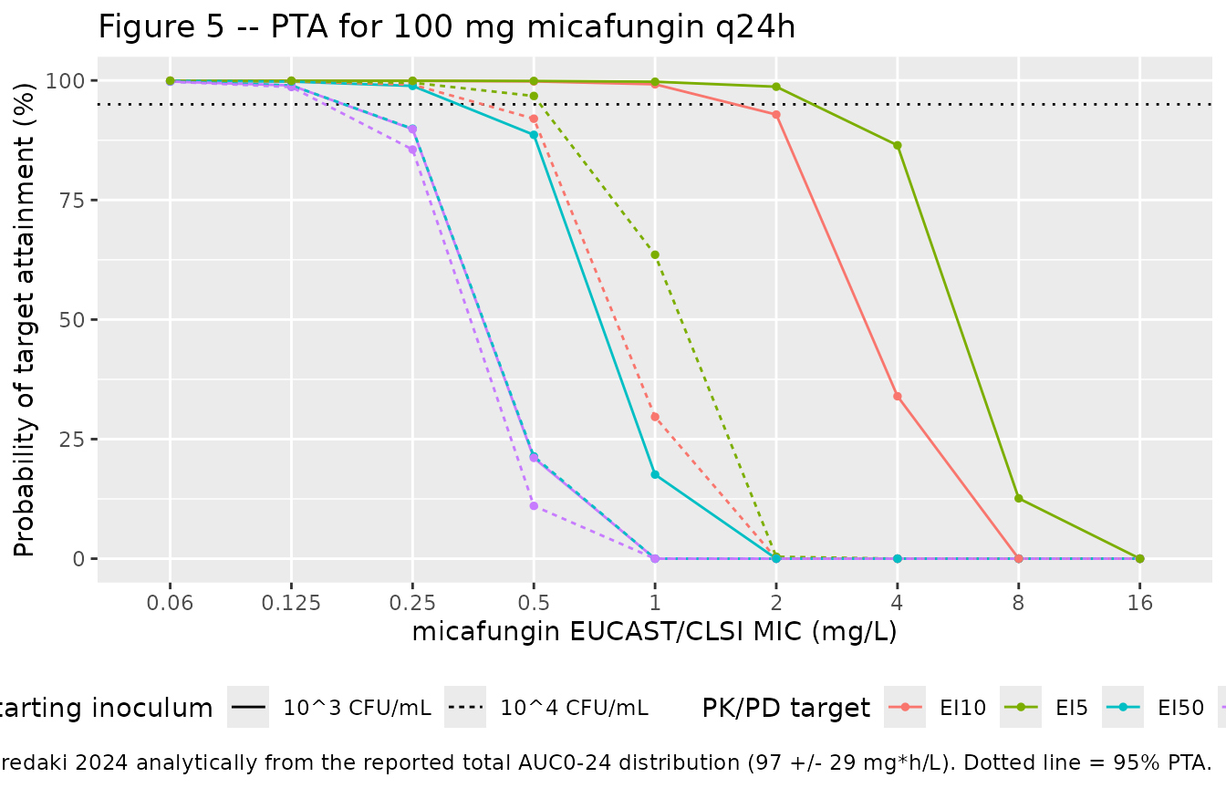
pta_tbl |>
  dplyr::filter(mic %in% c(0.25, 0.5, 1, 2, 4)) |>
  dplyr::mutate(pta = round(pta, 1)) |>
  dplyr::select(inoculum, endpoint, mic, pta) |>
  tidyr::pivot_wider(names_from = mic, values_from = pta, names_prefix = "MIC ") |>
  dplyr::rename("Inoculum" = inoculum, "Target" = endpoint) |>
knitr::kable(caption = "Analytic PTA (%) at selected MICs, using the packaged serum curves' targets.")| Inoculum | Target | MIC 0.25 | MIC 0.5 | MIC 1 | MIC 2 | MIC 4 |
|---|---|---|---|---|---|---|
| 10^4 CFU/mL | stasis | 85.5 | 11.0 | 0.0 | 0.0 | 0.0 |
| 10^4 CFU/mL | EI50 | 89.9 | 21.4 | 0.0 | 0.0 | 0.0 |
| 10^4 CFU/mL | EI10 | 99.1 | 92.0 | 29.6 | 0.0 | 0.0 |
| 10^4 CFU/mL | EI5 | 99.5 | 96.8 | 63.6 | 0.4 | 0.0 |
| 10^3 CFU/mL | stasis | 89.8 | 21.1 | 0.0 | 0.0 | 0.0 |
| 10^3 CFU/mL | EI50 | 98.9 | 88.6 | 17.6 | 0.0 | 0.0 |
| 10^3 CFU/mL | EI10 | 99.9 | 99.8 | 99.2 | 92.9 | 34.0 |
| 10^3 CFU/mL | EI5 | 99.9 | 99.9 | 99.7 | 98.7 | 86.4 |
pta_at <- function(ino, ep, mic_val) {
  pta_tbl$pta[pta_tbl$inoculum == ino & pta_tbl$endpoint == ep & pta_tbl$mic == mic_val]
}
# The packaged targets and the Table 1 targets give the same PTA curves.
stopifnot(max(abs(pta_tbl$pta - pta_tbl$pta_table1)) < 5)
# Results: stasis PTA 86%, 10% and 0% at MICs 0.25, 0.5 and >= 1 mg/L for both
# inocula. The 10^3 stasis target (240) gives about 21% at 0.5 mg/L under the
# closed form whichever source supplies it, hence the looser bound there.
for (ino in c("10^4 CFU/mL", "10^3 CFU/mL")) {
  stopifnot(
    pta_at(ino, "stasis", 0.25) > 80, pta_at(ino, "stasis", 0.25) < 92,
    pta_at(ino, "stasis", 0.5) < 25,
    pta_at(ino, "stasis", 1) < 1
  )
}
stopifnot(pta_at("10^4 CFU/mL", "stasis", 0.5) < 15)
# Results: EI10 at 10^3 CFU/mL gives high PTA for susceptible isolates.
stopifnot(pta_at("10^3 CFU/mL", "EI10", 1) > 99, pta_at("10^3 CFU/mL", "EI10", 2) > 90)
The stasis-target PTAs reproduce the 86% / 10% / 0% the Results quote at MICs of 0.25, 0.5 and >= 1 mg/L for the 10^4 CFU/mL inoculum. For 10^3 CFU/mL the closed form gives 89.8% and 21.1% at 0.25 and 0.5 mg/L, and the paper’s own Table 1 stasis target (240) gives 21.4% at 0.5 mg/L as well. For the proposed EI10 target at 10^3 CFU/mL the analytic PTA at the breakpoint MIC of 2 mg/L is 92.9%, a few points below the >= 95% shown in Figure 5(c); the paper’s own Table 1 value of 28 tAUC0-24/MIC gives 92.1% under the same calculation, so the gap is in the Monte Carlo procedure (not described beyond “the normal random number generator function of Excel”), not in the packaged curve.
Assumptions and deviations
- Four files, one per fitted curve. Beredaki 2024 fitted the exposure-response separately for each medium and starting inoculum, and reports that the Emin and n of the two serum curves differ significantly (P = 0.04). Each fitted curve is therefore its own model file.
- The printed Hill coefficient of the 10^3 CFU/mL serum curve is treated as a typesetting error. Results print “the Emin (4 versus 5.23) and n (-2.9 versus -1.15)”. With Emin 5.23, the constrained Emax -2 and the published EI50 124, n = 1.15 gives stasis, EI10 and EI5 of 286, 18 and 10 tAUC0-24/MIC against the Table 1 values 240, 28 and 16. n = 1.45 reproduces all three to within 3% (table above), and an independent least-squares trace of the drawn curve in Figure 4 gives n = 1.48 (with Emin 5.24 and EI50 126 tAUC0-24/MIC, confirming the other two published coefficients). The packaged model uses 1.45. The 10^4 CFU/mL curve’s printed coefficients (Emin 4, EI50 240, n 2.9) reproduce both Table 1 and the drawn curve and are used as published.
- The serum-free exposure-response coefficients were digitised from Figure 4. The paper prints Emin and n only for the serum curves. For the two RPMI curves the fitted lines in the right panel of Figure 4 were traced from the 200 dpi figure embedded in the publisher PDF, calibrated on the labelled decade ticks of the log10 x-axis and the y-axis ticks, and the published equation was least-squares fitted with Emax held at its constrained value (-3 or -2). Residual RMSE was 0.027 (10^4) and 0.037 (10^3) log10 CFU/mL. The recovered curves reproduce Table 1’s stasis, EI10 and EI5 within 12%, but their EI50s (25.1 and 41.3 fAUC0-24/MIC) are 7% and 11% below Table 1’s (27 and 46). No single curve with the drawn Emin can match all four Table 1 values – with EI50 fixed at 46, the stasis and EI10 targets would require Emin of about 2.8 for the 10^3 curve, against a plotted top asymptote of 4.4 and a control growth of 4.7 log10 CFU/mL – so the drawn curve was taken as the authority.
- Index scales. The serum models are indexed on total AUC0-24/MIC, as in the paper’s Methods and Table 1. The serum-free models are indexed on the AUC in the protein-free medium, which is fAUC0-24/MIC; Table 1’s tAUC figures for RPMI are this value divided by 0.0025. Figure 4 plots both media on the fAUC axis.
-
cmaxto AUC0-24 uses the idealised PK. The model converts the target peak into the index analytically from the achieved mono-exponential half-life. The paper calculated each experiment’s AUC0-24 from the measured profiles, which scatter around the targets (Figure 1). The exposure-response relationship – the part the paper fitted – is unaffected, which is why the Table 1 validation above is done on the index axis; time-kill endpoints at a given nominal Cmax can differ from Figures 2 and 3 by the scatter of the measured exposure. -
log10_cfu0uses the measured rather than the nominal inoculum. The mean t = 0 densities of the drug-free controls (4.28 / 3.2 with serum, 3.94 / 3.06 in RPMI) are used so the simulated trajectories start where the figures do. Only the offset is affected; the model describes the change in log10 CFU/mL. - Linear 72 h trajectory. Only the 72 h change was fitted, so the model spreads it uniformly over the window. The intermediate time points of Figures 2 and 3 (lag phases, early killing) are not described.
-
Residual error and variability. The paper reports
no assay CV and only R^2 for the exposure-response fits, so
propSdandaddSd_log10cfuare fixed at 0 and the models are for deterministic typical-value simulation. The in vitro experiment has no hierarchical structure and no eta parameters. - The PTA replication is analytic, not Monte Carlo. The paper drew 5000 patients from a normal total-AUC0-24 distribution in Excel; the closed form is used so the vignette is deterministic.
- Not packaged. The pan-echinocandin-resistant isolate (no effect at any exposure) and the static serum-growth screen of 20 isolates have no fitted model in the paper.