Propofol BIS and cAAI in adolescents (Blusse van Oud-Alblas 2019)
Source:vignettes/articles/BlussevanOudAlblas_2019_propofol.Rmd
BlussevanOudAlblas_2019_propofol.RmdModel and source
This paper contributes two model files, one per pharmacodynamic endpoint. The authors fitted a single two-compartment propofol pharmacokinetic model and then fitted each endpoint’s pharmacodynamic model sequentially to the post hoc pharmacokinetic parameters, so each file is a self-contained PK-PD model that carries the same PK block and a different biophase plus sigmoid Emax layer.
- Article: https://doi.org/10.1186/s12871-019-0684-z (BMC Anesthesiology 19:15; PMCID PMC6343297)
mod_bis <- rxode2::rxode2(readModelDb("BlussevanOudAlblas_2019_propofol_bis"))
#> ℹ parameter labels from comments will be replaced by 'label()'
mod_caai <- rxode2::rxode2(readModelDb("BlussevanOudAlblas_2019_propofol_caai"))
#> ℹ parameter labels from comments will be replaced by 'label()'- Citation: Blusse van Oud-Alblas HJ, Brill MJE, Peeters MYM, Tibboel D, Danhof M, Knibbe CAJ. (2019). Population pharmacokinetic-pharmacodynamic model of propofol in adolescents undergoing scoliosis surgery with intraoperative wake-up test: a study using Bispectral index and composite auditory evoked potentials as pharmacodynamic endpoints. BMC Anesthesiology 19:15. doi:10.1186/s12871-019-0684-z. PMCID: PMC6343297.
Bispectral Index (BIS) model – Population PK-PD model for propofol in adolescents undergoing idiopathic scoliosis surgery with an intraoperative wake-up test and reinduction of anesthesia (Blusse van Oud-Alblas 2019). A two-compartment whole-blood disposition model (CL 1.37 L/min, V1 3.6 L, Q 1.15 L/min, V2 76.8 L) is linked to a TWO-compartment biophase (effect-site) distribution model and an inhibitory sigmoid Emax model for the Bispectral Index (BIS). The central biophase compartment equilibrates with whole-blood propofol at ke0 = 0.102 1/min and exchanges with a peripheral biophase compartment at ke12 = 0.121 and ke21 = 0.172 1/min; the two-compartment biophase gave a time to peak effect-site concentration of 2.63 min and was superior to a one-compartment biophase (p < 0.001). BIS baseline and Emax were both fixed to 100 because too few awake observations were available to estimate them. No covariate (bodyweight, age, gender or remifentanil infusion rate) reached significance on any PK or PD parameter. The companion model for the composite A-line ARX index endpoint of the same study is modellib(‘BlussevanOudAlblas_2019_propofol_caai’).
Composite A-line ARX Index (cAAI) model – Population PK-PD model for propofol in adolescents undergoing idiopathic scoliosis surgery with an intraoperative wake-up test and reinduction of anesthesia (Blusse van Oud-Alblas 2019). A two-compartment whole-blood disposition model (CL 1.37 L/min, V1 3.6 L, Q 1.15 L/min, V2 76.8 L) is linked to a ONE-compartment biophase (effect-site) distribution model (ke0 = 0.067 1/min) and an inhibitory sigmoid Emax model for the composite A-line ARX index (cAAI); a two-compartment biophase was not superior for this endpoint (P > 0.05). The cAAI baseline was estimated at 63.4 and the maximum propofol effect at 0.786 of baseline, so cAAI falls to about 13.6 at saturating effect-site concentrations. The very steep Hill coefficient of 6.85 reproduces the near on-off cAAI response the authors observed at emergence, and contrasts with the gradual BIS response of the companion model modellib(‘BlussevanOudAlblas_2019_propofol_bis’). No covariate (bodyweight, age, gender or remifentanil infusion rate) reached significance on any PK or PD parameter.
data.frame(
  model = c("BIS", "cAAI"),
  states = c(paste(mod_bis$state, collapse = ", "), paste(mod_caai$state, collapse = ", "))
) |>
  dplyr::rename("Model" = model, "ODE states" = states) |>
knitr::kable()| Model | ODE states |
|---|---|
| BIS | central, peripheral1, effect1, effect2 |
| cAAI | central, peripheral1, effect |
Population
Fourteen ASA physical status I-II adolescents undergoing surgical correction of idiopathic scoliosis with an intraoperative wake-up test and reinduction of anesthesia, at the Erasmus University Medical Center (Rotterdam, the Netherlands). Baseline characteristics are reproduced from Table 1 of the paper and are reported as median (minimum-maximum).
tibble::tribble(
  ~characteristic, ~value,
  "Subjects (n)", "14",
  "Sex (male / female)", "2 / 12",
  "Age (years)", "14.7 (9.8 - 20.1)",
  "Bodyweight (kg)", "51 (36.6 - 82)",
  "Height (cm)", "162.5 (142 - 183)",
  "Blood samples per patient", "16 (6 - 22)",
  "BIS observations per patient", "113 (66 - 154)",
  "cAAI observations per patient", "100 (60 - 141)",
  "Duration of propofol infusion (min)", "410.0 (200 - 460)",
  "Length of wake-up test (min)", "21.5 (7.6 - 42.4)",
  "Return of consciousness after infusion (min)", "52.2 (22.6 - 116.33)"
) |>
  dplyr::rename("Characteristic" = characteristic, "Median (min - max)" = value) |>
knitr::kable()| Characteristic | Median (min - max) |
|---|---|
| Subjects (n) | 14 |
| Sex (male / female) | 2 / 12 |
| Age (years) | 14.7 (9.8 - 20.1) |
| Bodyweight (kg) | 51 (36.6 - 82) |
| Height (cm) | 162.5 (142 - 183) |
| Blood samples per patient | 16 (6 - 22) |
| BIS observations per patient | 113 (66 - 154) |
| cAAI observations per patient | 100 (60 - 141) |
| Duration of propofol infusion (min) | 410.0 (200 - 460) |
| Length of wake-up test (min) | 21.5 (7.6 - 42.4) |
| Return of consciousness after infusion (min) | 52.2 (22.6 - 116.33) |
Anesthesia was induced with a 4 mg/kg propofol bolus given over 10 s and maintained with a 2-10 mg/kg/h propofol infusion, alongside remifentanil (1 ug/kg/min at induction, then 0.2-1 ug/kg/min). For the wake-up test both infusions were stopped; after the test patients were reanesthetized with a 3-5 mg/kg propofol bolus and maintenance was resumed. Propofol was measured in whole blood by HPLC with fluorescence detection (limit of quantification 0.005 mg/L), so every concentration in this vignette is a whole-blood concentration.
None of the screened covariates (bodyweight, age, gender,
remifentanil infusion rate) reached significance on any pharmacokinetic
or pharmacodynamic parameter, so both model files carry an empty
covariateData and record the screen in
covariatesDataExcluded.
Source trace
Every ini() value and every model()
equation, with its location in the source article.
tibble::tribble(
  ~parameter, ~value, ~source,
  "lcl", "log(1.37) L/min", "Table 2, CL = 1.37 (CV 7.0%)",
  "lvc", "log(3.6) L", "Table 2, V1 = 3.6 (CV 10.2%)",
  "lq", "log(1.15) L/min", "Table 2, Q = 1.15 (CV 29.4%)",
  "lvp", "log(76.8) L", "Table 2, V2 = 76.8 (CV 5.0%)",
  "etalcl", "0.0476857", "Table 2, 'omega^2 of CL in %' = 22.1; log(1 + 0.221^2)",
  "propSd", "0.19", "Table 2, sigma^2 = 19.0%; Eq. 2 is additive on the log scale",
  "d/dt(central), d/dt(peripheral1)", "CL / V1 / Q / V2 micro-constants", "Pharmacokinetic model section (NONMEM ADVAN3 TRANS4)",
  "Cc <- central / vc", "whole-blood concentration (mg/L)", "Blood sampling and analysis section"
) |>
  dplyr::rename("Parameter / equation" = parameter, "Value" = value, "Source" = source) |>
knitr::kable(caption = "Pharmacokinetic block, shared by both model files.")| Parameter / equation | Value | Source |
|---|---|---|
| lcl | log(1.37) L/min | Table 2, CL = 1.37 (CV 7.0%) |
| lvc | log(3.6) L | Table 2, V1 = 3.6 (CV 10.2%) |
| lq | log(1.15) L/min | Table 2, Q = 1.15 (CV 29.4%) |
| lvp | log(76.8) L | Table 2, V2 = 76.8 (CV 5.0%) |
| etalcl | 0.0476857 | Table 2, ‘omega^2 of CL in %’ = 22.1; log(1 + 0.221^2) |
| propSd | 0.19 | Table 2, sigma^2 = 19.0%; Eq. 2 is additive on the log scale |
| d/dt(central), d/dt(peripheral1) | CL / V1 / Q / V2 micro-constants | Pharmacokinetic model section (NONMEM ADVAN3 TRANS4) |
| Cc <- central / vc | whole-blood concentration (mg/L) | Blood sampling and analysis section |
tibble::tribble(
  ~parameter, ~bis, ~caai, ~source,
  "le0", "fixed(log(100))", "log(63.4)", "Table 3, E0 row (BIS '100 Fixed'; cAAI 63.4, CV 14.9%)",
  "limax", "fixed(log(100))", "log(0.786)", "Table 3, 'Emax (value)' for BIS; 'Emax (fraction of E0)' for cAAI",
  "lec50", "log(3.51)", "log(2.14)", "Table 3, EC50 (mg/l)",
  "lhill", "log(1.43)", "log(6.85)", "Table 3, gamma",
  "lke0", "log(0.102)", "log(0.067)", "Table 3, k_eo (min^-1)",
  "lke12", "log(0.121)", "not in the cAAI model", "Table 3, k_e12",
  "lke21", "log(0.172)", "not in the cAAI model", "Table 3, k_e21",
  "etalec50", "0.059", "0.159", "Table 3, omega_EC50^2",
  "etalhill", "0.117", "0.952", "Table 3, omega_gamma^2",
  "etalke0", "0.192", "0.498", "Table 3, omega_keo^2",
  "addSd", "sqrt(59.5) = 7.7136", "sqrt(133) = 11.5326", "Table 3, sigma^2; Eq. 5 is additive on the index scale",
  "biophase ODEs", "two-compartment (effect1, effect2)", "one-compartment (effect), Eq. 3", "Fig. 1 caption and Pharmacodynamic model section",
  "sigmoid Emax", "E0 - Emax * Ce^g / (EC50^g + Ce^g)", "same, with Emax = fraction * E0", "Eq. 4"
) |>
  dplyr::rename(
    "Parameter / equation" = parameter, "BIS model" = bis,
    "cAAI model" = caai, "Source" = source
  ) |>
knitr::kable(caption = "Pharmacodynamic blocks of the two model files.")| Parameter / equation | BIS model | cAAI model | Source |
|---|---|---|---|
| le0 | fixed(log(100)) | log(63.4) | Table 3, E0 row (BIS ‘100 Fixed’; cAAI 63.4, CV 14.9%) |
| limax | fixed(log(100)) | log(0.786) | Table 3, ‘Emax (value)’ for BIS; ‘Emax (fraction of E0)’ for cAAI |
| lec50 | log(3.51) | log(2.14) | Table 3, EC50 (mg/l) |
| lhill | log(1.43) | log(6.85) | Table 3, gamma |
| lke0 | log(0.102) | log(0.067) | Table 3, k_eo (min^-1) |
| lke12 | log(0.121) | not in the cAAI model | Table 3, k_e12 |
| lke21 | log(0.172) | not in the cAAI model | Table 3, k_e21 |
| etalec50 | 0.059 | 0.159 | Table 3, omega_EC50^2 |
| etalhill | 0.117 | 0.952 | Table 3, omega_gamma^2 |
| etalke0 | 0.192 | 0.498 | Table 3, omega_keo^2 |
| addSd | sqrt(59.5) = 7.7136 | sqrt(133) = 11.5326 | Table 3, sigma^2; Eq. 5 is additive on the index scale |
| biophase ODEs | two-compartment (effect1, effect2) | one-compartment (effect), Eq. 3 | Fig. 1 caption and Pharmacodynamic model section |
| sigmoid Emax | E0 - Emax * Ce^g / (EC50^g + Ce^g) | same, with Emax = fraction * E0 | Eq. 4 |
Two readings of the source tables are load-bearing and were cross-checked against the paper’s own prose:
-
Table 2 reports the CL inter-individual variability already
back-transformed. Its footnote defines the printed percentage
as
sqrt(exp(omega^2) - 1), so22.1is a 22.1% CV and the log-scale variance stored inini()islog(1 + 0.221^2) = 0.0476857. -
Table 3 reports the pharmacodynamic terms as the variances
themselves. The Results text back-transforms three of them
explicitly, which confirms the reading:
0.059is quoted as “a CV of 25%”,0.159as “CV 42%”, and0.952as “CV = 126%”.
omega2 <- c(
  "BIS EC50" = 0.059, "BIS gamma" = 0.117,
  "cAAI EC50" = 0.159, "cAAI gamma" = 0.952
)
tibble::tibble(
  term = names(omega2),
  variance = omega2,
  cv_pct = round(100 * sqrt(exp(omega2) - 1), 1),
  paper_cv_pct = c(25, 34, 42, 126)
) |>
  dplyr::rename(
    "Term" = term, "Table 3 omega^2" = variance,
    "Back-transformed CV (%)" = cv_pct, "CV quoted in Results (%)" = paper_cv_pct
  ) |>
knitr::kable()| Term | Table 3 omega^2 | Back-transformed CV (%) | CV quoted in Results (%) |
|---|---|---|---|
| BIS EC50 | 0.059 | 24.7 | 25 |
| BIS gamma | 0.117 | 35.2 | 34 |
| cAAI EC50 | 0.159 | 41.5 | 42 |
| cAAI gamma | 0.952 | 126.1 | 126 |
Structural check: time to peak effect-site concentration
The paper reports a single number that depends on the whole linked system – the pharmacokinetic disposition, the biophase topology, and all three biophase rate constants together:
The Tmax of the two-compartment biophase distribution model was 2.63 min.
This is the time at which the concentration in the central effect-site compartment peaks after a bolus dose, and it is the sharpest available check that the two-compartment biophase was transcribed correctly. The equations for the two-compartment biophase are not printed in the article (only Eq. 3, the one-compartment form, is), so this check is what pins the structure that was reconstructed from the Fig. 1 caption.
bolus_events <- function(dose_mg, times) {
  rbind(
    data.frame(
      id = 1L, time = 0, amt = dose_mg, rate = 0,
      evid = 1L, cmt = "central"
    ),
    data.frame(
      id = 1L, time = times, amt = NA_real_, rate = NA_real_,
      evid = 0L, cmt = "Cc"
    )
  )
}

# 0.005 min resolution so the peak can be located to the two decimal places
# the paper reports.
tp_times <- seq(0, 20, by = 0.005)
tp_ev <- bolus_events(200, tp_times)

# omega = NA / sigma = NA gives the typical-value (no random effects) profile.
tp_bis <- rxode2::rxSolve(
  mod_bis, tp_ev,
  returnType = "data.frame", useLinCmt = FALSE, omega = NA, sigma = NA
)
tp_caai <- rxode2::rxSolve(
  mod_caai, tp_ev,
  returnType = "data.frame", useLinCmt = FALSE, omega = NA, sigma = NA
)
A one-compartment biophase carrying the same
ke0 is simulated alongside it, to show that the reported
2.63 min is not reachable without the peripheral effect compartment.
# Same PK, same ke0 = 0.102, but the one-compartment biophase of Eq. 3. Built
# by setting ke12 = ke21 = 0 in the BIS model, which collapses the two-
# compartment biophase to Eq. 3 exactly.
tp_bis_1cmt <- rxode2::rxSolve(
  mod_bis, tp_ev,
  params = c(lke12 = log(1e-12), lke21 = log(1e-12)),
  returnType = "data.frame", useLinCmt = FALSE, omega = NA, sigma = NA
)

tpeak <- c(
  bis_2cmt = tp_bis$time[which.max(tp_bis$effect1)],
  bis_1cmt = tp_bis_1cmt$time[which.max(tp_bis_1cmt$effect1)],
  caai_1cmt = tp_caai$time[which.max(tp_caai$effect)]
)

tibble::tibble(
  structure = c(
    "BIS, two-compartment biophase (ke0 0.102, ke12 0.121, ke21 0.172)",
    "BIS ke0 only, one-compartment biophase (Eq. 3)",
    "cAAI, one-compartment biophase (ke0 0.067, Eq. 3)"
  ),
  tmax_min = round(unname(tpeak), 3),
  reported = c("2.63 (Results)", "not reported", "not reported")
) |>
  dplyr::rename(
    "Biophase structure" = structure, "Simulated Tmax (min)" = tmax_min,
    "Reported in the paper" = reported
  ) |>
knitr::kable()| Biophase structure | Simulated Tmax (min) | Reported in the paper |
|---|---|---|
| BIS, two-compartment biophase (ke0 0.102, ke12 0.121, ke21 0.172) | 2.630 | 2.63 (Results) |
| BIS ke0 only, one-compartment biophase (Eq. 3) | 3.300 | not reported |
| cAAI, one-compartment biophase (ke0 0.067, Eq. 3) | 3.835 | not reported |
# Structural gate. This is a deterministic typical-value solve, so there is no
# cohort randomness to guard against: the tolerance is numerical only (the peak
# can only be located to the 0.005 min grid resolution, and the paper prints
# two decimals).
stopifnot(abs(tpeak[["bis_2cmt"]] - 2.63) <= 0.01)
dplyr::bind_rows(
  tp_bis |> dplyr::transmute(time, ce = effect1, structure = "Two-compartment biophase (BIS)"),
  tp_bis_1cmt |> dplyr::transmute(time, ce = effect1, structure = "One-compartment biophase, same ke0"),
  tp_caai |> dplyr::transmute(time, ce = effect, structure = "One-compartment biophase (cAAI)")
) |>
  ggplot2::ggplot(ggplot2::aes(time, ce, colour = structure, linetype = structure)) +
  ggplot2::geom_line() +
  ggplot2::geom_vline(xintercept = 2.63, colour = "grey40", linetype = "dotted") +
  ggplot2::annotate("text", x = 2.63, y = Inf, label = " reported Tmax 2.63 min",
                    hjust = 0, vjust = 1.5, size = 3, colour = "grey30") +
  ggplot2::labs(
    x = "Time after bolus (min)", y = "Effect-site concentration (mg/L)",
    colour = NULL, linetype = NULL
  ) +
  ggplot2::theme_bw() +
  ggplot2::theme(legend.position = "bottom", legend.direction = "vertical")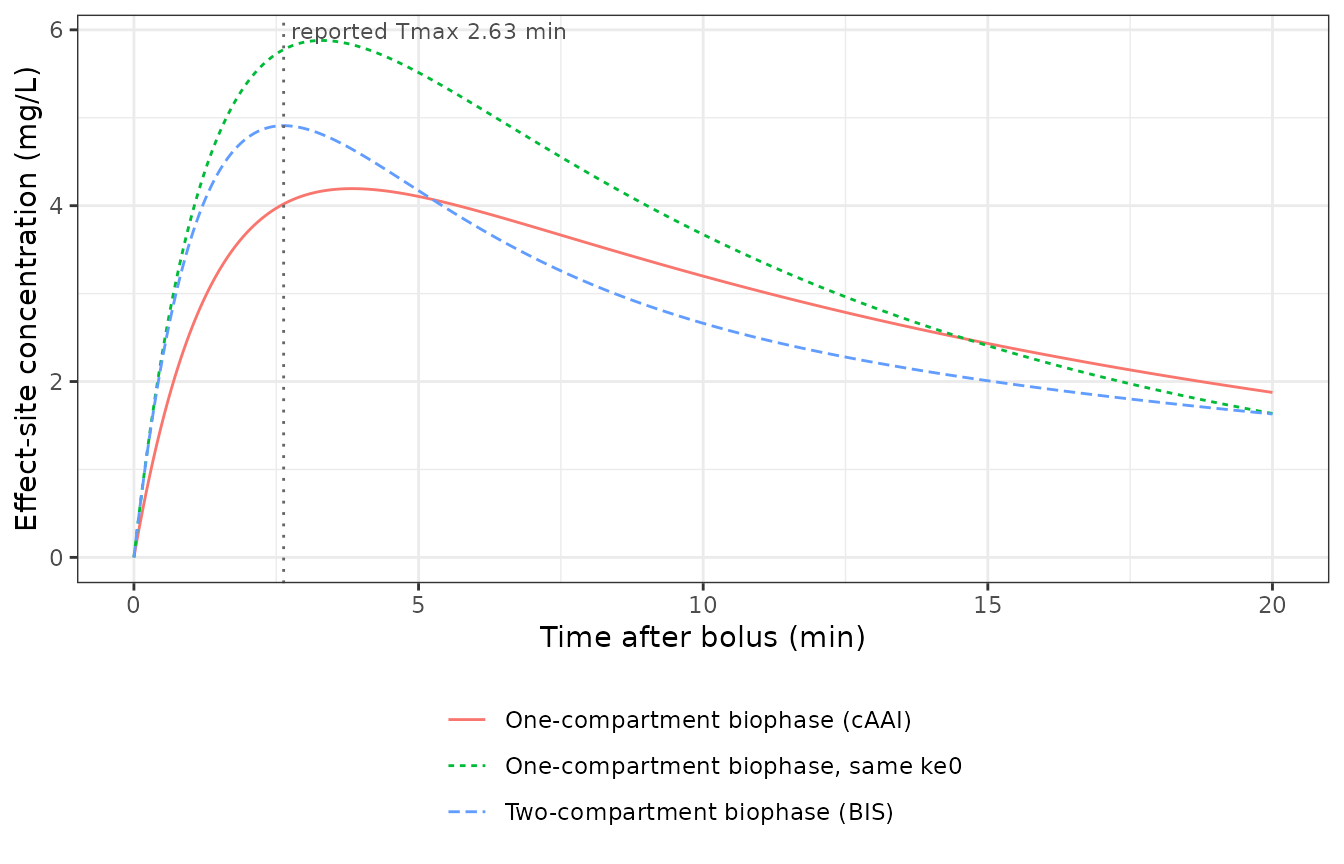
Effect-site concentration after a 200 mg propofol bolus. The two-compartment biophase (solid) peaks at the 2.63 min reported by the paper; the one-compartment biophase with the same ke0 (dashed) peaks later and decays faster.
Structural check: the cAAI baseline, Emax and floor
Table 3 reports the cAAI maximum effect as a fraction of the baseline (0.786), and the Results text then states the two derived quantities. Both are reproduced exactly by the packaged model.
e0_caai <- 63.4
frac_caai <- 0.786

# Asymptotic cAAI: solve at a saturating effect-site concentration.
caai_floor <- e0_caai * (1 - frac_caai)

tibble::tibble(
  quantity = c(
    "Emax on the cAAI scale",
    "cAAI at saturating effect-site concentration"
  ),
  computed = round(c(frac_caai * e0_caai, caai_floor), 2),
  reported = c("49.8 (Results)", "14 (Results, 'a maximum effect of 14')")
) |>
  dplyr::rename(
    "Quantity" = quantity, "Computed from Table 3" = computed,
    "Reported in the paper" = reported
  ) |>
knitr::kable()| Quantity | Computed from Table 3 | Reported in the paper |
|---|---|---|
| Emax on the cAAI scale | 49.83 | 49.8 (Results) |
| cAAI at saturating effect-site concentration | 13.57 | 14 (Results, ‘a maximum effect of 14’) |
Replicating Figure 4: concentration-effect relationships
Figure 4 of the paper plots BIS and cAAI against propofol concentration for the final models, and the Results narrative describes what to look for: “BIS values gradually change as a result of the propofol concentration, while for cAAI a more rapid change in values are observed as a result of the higher Hill coefficient.”
Both curves are Eq. 4 evaluated at equilibrium, where the effect-site concentration equals the blood concentration.
ce_grid <- seq(0, 10, length.out = 401)

curve_df <- dplyr::bind_rows(
  tibble::tibble(
    ce = ce_grid,
    index = 100 - 100 * ce_grid^1.43 / (3.51^1.43 + ce_grid^1.43),
    endpoint = "BIS"
  ),
  tibble::tibble(
    ce = ce_grid,
    index = e0_caai * (1 - frac_caai * ce_grid^6.85 / (2.14^6.85 + ce_grid^6.85)),
    endpoint = "cAAI"
  )
)

ggplot2::ggplot(curve_df, ggplot2::aes(ce, index, linetype = endpoint)) +
  ggplot2::geom_line() +
  ggplot2::scale_linetype_manual(values = c(BIS = "solid", cAAI = "dotted")) +
  ggplot2::labs(
    x = "Propofol effect-site concentration (mg/L)",
    y = "BIS or cAAI value", linetype = NULL
  ) +
  ggplot2::theme_bw()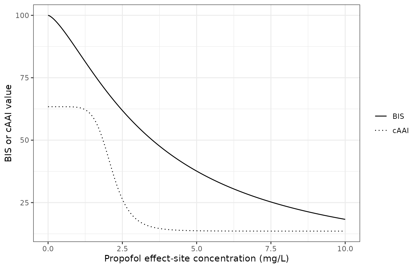
Replicates Figure 4 of Blusse van Oud-Alblas 2019: propofol concentration-effect relation for BIS (solid) and cAAI (dotted) for the final models.
The EC50 definition provides a closed-form check on each curve: at
Ce = EC50 the index must have fallen by exactly half of its
Emax.
bis_at_ec50 <- 100 - 100 * 3.51^1.43 / (3.51^1.43 + 3.51^1.43)
caai_at_ec50 <- e0_caai * (1 - frac_caai * 2.14^6.85 / (2.14^6.85 + 2.14^6.85))

tibble::tibble(
  endpoint = c("BIS", "cAAI"),
  ec50 = c(3.51, 2.14),
  index_at_ec50 = round(c(bis_at_ec50, caai_at_ec50), 3),
  expected = round(c(100 - 100 / 2, e0_caai * (1 - frac_caai / 2)), 3)
) |>
  dplyr::rename(
    "Endpoint" = endpoint, "EC50 (mg/L)" = ec50,
    "Index at EC50" = index_at_ec50, "E0 - Emax / 2" = expected
  ) |>
knitr::kable()| Endpoint | EC50 (mg/L) | Index at EC50 | E0 - Emax / 2 |
|---|---|---|---|
| BIS | 3.51 | 50.000 | 50.000 |
| cAAI | 2.14 | 38.484 | 38.484 |
The steepness contrast the authors emphasise is quantified by the width of the concentration band over which each index travels from 80% to 20% of its full range – a factor of nearly five between the two monitors.
band_width <- function(hill, ec50) {
  # Ce at which the sigmoid fraction equals p is ec50 * (p / (1 - p))^(1 / hill)
  ec50 * ((0.8 / 0.2)^(1 / hill) - (0.2 / 0.8)^(1 / hill))
}

tibble::tibble(
  endpoint = c("BIS", "cAAI"),
  hill = c(1.43, 6.85),
  width = round(c(band_width(1.43, 3.51), band_width(6.85, 2.14)), 2)
) |>
  dplyr::rename(
    "Endpoint" = endpoint, "Hill coefficient" = hill,
    "Ce width from 20% to 80% of Emax (mg/L)" = width
  ) |>
knitr::kable()| Endpoint | Hill coefficient | Ce width from 20% to 80% of Emax (mg/L) |
|---|---|---|
| BIS | 1.43 | 7.92 |
| cAAI | 6.85 | 0.87 |
Replicating Figure 3: a simulated surgical course with a wake-up test
Figure 3 of the paper shows propofol concentration (3a), BIS (3b) and cAAI (3c) against time in a representative adolescent through induction, maintenance, the intraoperative wake-up test, reinduction and emergence. The event table below reproduces that sequence for a 51 kg adolescent – the cohort median weight – using the protocol doses from the Methods. The maintenance phase is shortened relative to the study’s 410 min median so the vignette renders quickly; the structure of the course is unchanged.
wt_median <- 51

t_wakeup_start <- 150 # stop the infusion for the wake-up test
t_wakeup_len <- 21.5 # Table 1 median length of the wake-up test
t_reind <- t_wakeup_start + t_wakeup_len
t_end <- 300 # end of surgery, infusions discontinued

bolus_min <- 10 / 60 # the protocol 10 s induction bolus
maint_rate <- 6 / 60 * wt_median # 6 mg/kg/h, mid-range of the 2-10 protocol

infusion_row <- function(id, start, stop, rate) {
  data.frame(
    id = id, time = start, amt = rate * (stop - start), rate = rate,
    evid = 1L, cmt = "central"
  )
}
bolus_row <- function(id, at, dose_mgkg, wt) {
  data.frame(
    id = id, time = at, amt = dose_mgkg * wt, rate = dose_mgkg * wt / bolus_min,
    evid = 1L, cmt = "central"
  )
}

obs_times <- sort(unique(c(
  seq(0, 400, by = 0.25),
  t_wakeup_start, t_reind, t_reind + bolus_min, t_end
)))

timeline_ev <- rbind(
  bolus_row(1L, 0, 4, wt_median), # induction, 4 mg/kg over 10 s
  infusion_row(1L, bolus_min, t_wakeup_start, maint_rate), # maintenance
  bolus_row(1L, t_reind, 4, wt_median), # reinduction, 3-5 mg/kg
  infusion_row(1L, t_reind + bolus_min, t_end, maint_rate), # maintenance resumed
  data.frame(
    id = 1L, time = obs_times, amt = NA_real_, rate = NA_real_,
    evid = 0L, cmt = "Cc"
  )
)
tl_bis <- rxode2::rxSolve(
  mod_bis, timeline_ev,
  returnType = "data.frame", useLinCmt = FALSE, omega = NA, sigma = NA
) |>
  dplyr::filter(!is.na(Cc))
tl_caai <- rxode2::rxSolve(
  mod_caai, timeline_ev,
  returnType = "data.frame", useLinCmt = FALSE, omega = NA, sigma = NA
) |>
  dplyr::filter(!is.na(Cc))
wake_band <- ggplot2::annotate(
  "rect",
  xmin = t_wakeup_start, xmax = t_reind, ymin = -Inf, ymax = Inf,
  fill = "grey85", alpha = 0.6
)

panel_df <- dplyr::bind_rows(
  tl_bis |> dplyr::transmute(time, value = Cc, panel = "a. Propofol, whole blood (mg/L)"),
  tl_bis |> dplyr::transmute(time, value = BIS, panel = "b. Bispectral Index"),
  tl_caai |> dplyr::transmute(time, value = cAAI, panel = "c. Composite A-line ARX Index")
)

ggplot2::ggplot(panel_df, ggplot2::aes(time, value)) +
  wake_band +
  ggplot2::geom_line() +
  ggplot2::facet_wrap(~panel, ncol = 1, scales = "free_y") +
  ggplot2::labs(x = "Time from induction (min)", y = NULL) +
  ggplot2::theme_bw()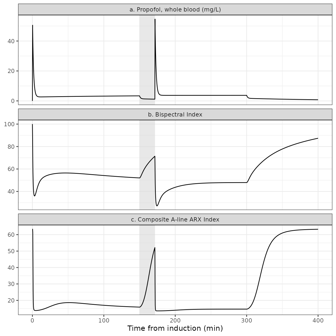
Replicates the structure of Figure 3 of Blusse van Oud-Alblas 2019 for a typical 51 kg adolescent: whole-blood propofol concentration (a), BIS (b) and cAAI (c) through induction, maintenance, the intraoperative wake-up test (shaded), reinduction and emergence.
Three qualitative features the paper describes are reproduced.
bis_wake <- max(tl_bis$BIS[tl_bis$time >= t_wakeup_start & tl_bis$time <= t_reind])
caai_wake <- max(tl_caai$cAAI[tl_caai$time >= t_wakeup_start & tl_caai$time <= t_reind])
bis_maint <- tl_bis$BIS[which.min(abs(tl_bis$time - (t_wakeup_start - 1)))]
caai_maint <- tl_caai$cAAI[which.min(abs(tl_caai$time - (t_wakeup_start - 1)))]

tibble::tibble(
  feature = c(
    "BIS just before the wake-up test",
    "Peak BIS during the wake-up test",
    "cAAI just before the wake-up test",
    "Peak cAAI during the wake-up test"
  ),
  simulated = round(c(bis_maint, bis_wake, caai_maint, caai_wake), 1),
  paper_reference = c(
    "target range under general anesthesia is 40 to 60",
    "values above 90 indicate wakefulness",
    "15 to 25 reflects surgical anesthesia",
    "levels higher than 45 indicate wakefulness"
  )
) |>
  dplyr::rename(
    "Feature" = feature, "Simulated" = simulated,
    "Monitor interpretation quoted in the paper" = paper_reference
  ) |>
knitr::kable()| Feature | Simulated | Monitor interpretation quoted in the paper |
|---|---|---|
| BIS just before the wake-up test | 52.1 | target range under general anesthesia is 40 to 60 |
| Peak BIS during the wake-up test | 71.4 | values above 90 indicate wakefulness |
| cAAI just before the wake-up test | 15.9 | 15 to 25 reflects surgical anesthesia |
| Peak cAAI during the wake-up test | 52.1 | levels higher than 45 indicate wakefulness |
# Both indices must rise during the wake-up test and fall again after
# reinduction; and maintenance BIS must sit in the anesthetic range the
# protocol targeted. These are structural, not cohort-extreme, assertions.
stopifnot(
  bis_wake > bis_maint,
  caai_wake > caai_maint,
  bis_maint > 30, bis_maint < 70,
  # The reinduction bolus must drive both indices back below their
  # pre-wake-up-test maintenance values.
  min(tl_bis$BIS[tl_bis$time > t_reind & tl_bis$time < t_end]) < bis_maint,
  min(tl_caai$cAAI[tl_caai$time > t_reind & tl_caai$time < t_end]) < caai_maint
)
The paper notes explicitly that the cAAI response is close to on-off while the BIS response is gradual; the simulated wake-up test shows the same contrast.
window <- tl_bis$time >= t_wakeup_start & tl_bis$time <= t_reind
tibble::tibble(
  endpoint = c("BIS", "cAAI"),
  rise = round(c(
    bis_wake - bis_maint,
    caai_wake - caai_maint
  ), 1),
  pct_of_range = round(100 * c(
    (bis_wake - bis_maint) / 100,
    (caai_wake - caai_maint) / (frac_caai * e0_caai)
  ), 1)
) |>
  dplyr::rename(
    "Endpoint" = endpoint, "Rise during the wake-up test" = rise,
    "Percent of the monitor's full drug effect range" = pct_of_range
  ) |>
knitr::kable()| Endpoint | Rise during the wake-up test | Percent of the monitor’s full drug effect range |
|---|---|---|
| BIS | 19.3 | 19.3 |
| cAAI | 36.2 | 72.7 |
Virtual cohort
A cohort of 100 adolescents is simulated with the model’s own random effects, using weights spanning the Table 1 range. The model carries no covariates, so weight enters only through the mg/kg protocol doses.
rxode2::rxSetSeed(20190115)
set.seed(20190115)

n_sub <- 100
cohort <- tibble::tibble(
  id = seq_len(n_sub),
  # Log-normal around the Table 1 median 51 kg, truncated to the observed
  # 36.6-82 kg range.
  WT = pmin(82, pmax(36.6, 51 * exp(stats::rnorm(n_sub, 0, 0.18))))
)

cohort_obs_times <- sort(unique(c(seq(0, 400, by = 1), t_wakeup_start, t_reind, t_end)))

cohort_dose_rows <- do.call(rbind, lapply(seq_len(n_sub), function(i) {
  wt <- cohort$WT[i]
  rate_i <- 6 / 60 * wt
  rbind(
    bolus_row(i, 0, 4, wt),
    infusion_row(i, bolus_min, t_wakeup_start, rate_i),
    bolus_row(i, t_reind, 4, wt),
    infusion_row(i, t_reind + bolus_min, t_end, rate_i)
  )
}))

cohort_obs_rows <- do.call(rbind, lapply(seq_len(n_sub), function(i) {
  data.frame(
    id = i, time = cohort_obs_times, amt = NA_real_, rate = NA_real_,
    evid = 0L, cmt = "Cc"
  )
}))

cohort_ev <- dplyr::bind_rows(cohort_dose_rows, cohort_obs_rows) |>
  dplyr::arrange(id, time, dplyr::desc(evid))

sim_bis <- rxode2::rxSolve(
  mod_bis, cohort_ev,
  returnType = "data.frame", useLinCmt = FALSE
) |>
  dplyr::filter(!is.na(Cc))
sim_caai <- rxode2::rxSolve(
  mod_caai, cohort_ev,
  returnType = "data.frame", useLinCmt = FALSE
) |>
  dplyr::filter(!is.na(Cc))
ribbon_df <- dplyr::bind_rows(
  sim_bis |> dplyr::transmute(time, value = Cc, panel = "a. Propofol, whole blood (mg/L)"),
  sim_bis |> dplyr::transmute(time, value = BIS, panel = "b. Bispectral Index"),
  sim_caai |> dplyr::transmute(time, value = cAAI, panel = "c. Composite A-line ARX Index")
) |>
  dplyr::group_by(panel, time) |>
  dplyr::summarise(
    lo = stats::quantile(value, 0.05),
    md = stats::median(value),
    hi = stats::quantile(value, 0.95),
    .groups = "drop"
  )

ggplot2::ggplot(ribbon_df, ggplot2::aes(time)) +
  wake_band +
  ggplot2::geom_ribbon(ggplot2::aes(ymin = lo, ymax = hi), fill = "steelblue", alpha = 0.3) +
  ggplot2::geom_line(ggplot2::aes(y = md)) +
  ggplot2::facet_wrap(~panel, ncol = 1, scales = "free_y") +
  ggplot2::labs(x = "Time from induction (min)", y = NULL) +
  ggplot2::theme_bw()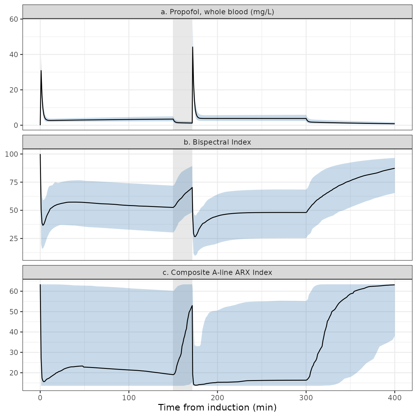
Simulated cohort of 100 adolescents (median and 5th-95th percentile band) through the same surgical course. The wake-up test window is shaded.
The cohort spread is dominated by the very large variability the
paper reports on the cAAI Hill coefficient
(omega^2 = 0.952, a CV of 126%), which is why the cAAI band
is far wider than the BIS band even though both share the same
pharmacokinetic model.
# Centre-of-distribution assertions only. The extremes of a simulated cohort
# are not reproducible across rxode2 versions (rxSetSeed fixes the draw within
# a version, not across versions), so nothing here asserts on a min or a max.
med_bis_maint <- stats::median(sim_bis$BIS[sim_bis$time == t_wakeup_start - 1])
med_caai_maint <- stats::median(sim_caai$cAAI[sim_caai$time == t_wakeup_start - 1])
med_bis_wake <- stats::median(sim_bis$BIS[sim_bis$time == t_reind])
med_caai_wake <- stats::median(sim_caai$cAAI[sim_caai$time == t_reind])

stopifnot(
  med_bis_maint > 30, med_bis_maint < 70,
  med_bis_wake > med_bis_maint,
  med_caai_wake > med_caai_maint
)
PKNCA validation of the pharmacokinetic block
The article reports no non-compartmental analysis, so the NCA is
validated against the closed-form identities of the published
two-compartment model instead of against a published NCA table.
For an intravenous bolus of dose D into a two-compartment
system these identities are exact:
-
AUC(0-inf) = D / CL, so the NCA-derived clearance must return CL = 1.37 L/min; -
Vss = V1 + V2 = 3.6 + 76.8 = 80.4 L, recoverable asD * AUMC / AUC^2; - the terminal half-life is
log(2) / beta, wherebetais the smaller eigenvalue of the disposition matrix built from CL / V1 / Q / V2.
Because the distribution phase of this model is extremely fast
(t1/2,alpha is about 1 min), the concentration grid is
densely sampled over the first minutes; without that, linear-trapezoidal
bias alone would produce an apparent several percent failure of a
correct model.
cl_pub <- 1.37
v1_pub <- 3.6
q_pub <- 1.15
v2_pub <- 76.8

k10 <- cl_pub / v1_pub
k12 <- q_pub / v1_pub
k21 <- q_pub / v2_pub
lam <- sort(Re(polyroot(c(k10 * k21, -(k10 + k12 + k21), 1))))
beta <- lam[1]

expected <- c(
  cl = cl_pub,
  vss = v1_pub + v2_pub,
  half_life = log(2) / beta
)
round(expected, 4)
#>        cl       vss half_life
#>    1.3700   80.4000   85.9878
nca_doses <- c(100, 200, 400)

# Dense early, then progressively coarser out to 600 min (about seven terminal
# half-lives) so lambda.z and the AUC extrapolation are well determined.
nca_times <- sort(unique(c(
  seq(0, 2, by = 0.005),
  seq(2, 10, by = 0.05),
  seq(10, 60, by = 0.5),
  seq(60, 600, by = 2)
)))

nca_ev <- do.call(rbind, lapply(seq_along(nca_doses), function(i) {
  rbind(
    data.frame(
      id = i, time = 0, amt = nca_doses[i], rate = 0,
      evid = 1L, cmt = "central"
    ),
    data.frame(
      id = i, time = nca_times, amt = NA_real_, rate = NA_real_,
      evid = 0L, cmt = "Cc"
    )
  )
}))

nca_sim <- rxode2::rxSolve(
  mod_bis, nca_ev,
  returnType = "data.frame", useLinCmt = FALSE, omega = NA, sigma = NA
)

nca_conc <- nca_sim |>
  dplyr::filter(!is.na(Cc)) |>
  dplyr::mutate(arm = paste0(nca_doses[id], " mg IV bolus")) |>
  dplyr::select(id, time, Cc, arm)

nca_dose <- nca_ev |>
  dplyr::filter(evid == 1L) |>
  dplyr::mutate(arm = paste0(nca_doses[id], " mg IV bolus")) |>
  dplyr::select(id, time, amt, arm)
conc_obj <- PKNCA::PKNCAconc(
  nca_conc, Cc ~ time | arm + id,
  concu = "mg/L", timeu = "min"
)
dose_obj <- PKNCA::PKNCAdose(
  nca_dose, amt ~ time | arm + id,
  doseu = "mg"
)

intervals <- data.frame(
  start = 0, end = Inf,
  cmax = TRUE, tmax = TRUE,
  aucinf.obs = TRUE, aumcinf.obs = TRUE,
  half.life = TRUE, lambda.z = TRUE,
  cl.obs = TRUE, vss.obs = TRUE, mrt.obs = TRUE
)

nca_res <- PKNCA::pk.nca(PKNCA::PKNCAdata(conc_obj, dose_obj, intervals = intervals))

arm_labels <- paste0(nca_doses, " mg IV bolus")

nca_wide <- as.data.frame(nca_res) |>
  dplyr::select(arm, PPTESTCD, PPORRES) |>
  tidyr::pivot_wider(names_from = PPTESTCD, values_from = PPORRES) |>
  # Join the dose back on by ARM LABEL, never by row position: pivot_wider and
  # PKNCA are both free to reorder groups.
  dplyr::left_join(
    tibble::tibble(arm = arm_labels, dose_mg = nca_doses),
    by = "arm"
  ) |>
  dplyr::arrange(dose_mg)
nca_wide |>
  dplyr::transmute(
    arm,
    dose_mg,
    cmax = round(cmax, 3),
    aucinf.obs = round(aucinf.obs, 2),
    cl.obs = round(cl.obs, 4),
    vss.obs = round(vss.obs, 2),
    half.life = round(half.life, 2)
  ) |>
  dplyr::rename(
    "Arm" = arm, "Dose (mg)" = dose_mg, "Cmax (mg/L)" = cmax,
    "AUC0-inf (mg*min/L)" = aucinf.obs, "CL (L/min)" = cl.obs,
    "Vss (L)" = vss.obs, "t1/2 (min)" = half.life
  ) |>
knitr::kable(caption = "PKNCA results from a typical-value simulation of the published model.")| Arm | Dose (mg) | Cmax (mg/L) | AUC0-inf (mg*min/L) | CL (L/min) | Vss (L) | t1/2 (min) |
|---|---|---|---|---|---|---|
| 100 mg IV bolus | 100 | 27.778 | 72.99 | 1.37 | 80.39 | 85.8 |
| 200 mg IV bolus | 200 | 55.556 | 145.99 | 1.37 | 80.39 | 85.8 |
| 400 mg IV bolus | 400 | 111.111 | 291.97 | 1.37 | 80.39 | 85.8 |
comparison <- tibble::tibble(
  parameter = c("CL (L/min)", "Vss (L)", "Terminal t1/2 (min)", "Cmax after 200 mg (mg/L)"),
  simulated = c(
    mean(nca_wide$cl.obs),
    mean(nca_wide$vss.obs),
    mean(nca_wide$half.life),
    nca_wide$cmax[nca_wide$dose_mg == 200]
  ),
  published = c(
    cl_pub,
    v1_pub + v2_pub,
    unname(expected[["half_life"]]),
    200 / v1_pub
  ),
  source = c(
    "Table 2, CL = 1.37 L/min",
    "Table 2, V1 + V2 = 3.6 + 76.8",
    "derived from Table 2 (smaller disposition eigenvalue)",
    "derived from Table 2 (D / V1 for an IV bolus)"
  )
) |>
  dplyr::mutate(pct_diff = 100 * (simulated - published) / published)

comparison |>
  dplyr::transmute(
    parameter,
    simulated = round(simulated, 3),
    published = round(published, 3),
    pct_diff = round(pct_diff, 2),
    source
  ) |>
  dplyr::rename(
    "NCA parameter" = parameter, "Simulated (PKNCA)" = simulated,
    "Published / closed form" = published, "Difference (%)" = pct_diff,
    "Source" = source
  ) |>
knitr::kable()| NCA parameter | Simulated (PKNCA) | Published / closed form | Difference (%) | Source |
|---|---|---|---|---|
| CL (L/min) | 1.370 | 1.370 | 0.00 | Table 2, CL = 1.37 L/min |
| Vss (L) | 80.391 | 80.400 | -0.01 | Table 2, V1 + V2 = 3.6 + 76.8 |
| Terminal t1/2 (min) | 85.798 | 85.988 | -0.22 | derived from Table 2 (smaller disposition eigenvalue) |
| Cmax after 200 mg (mg/L) | 55.556 | 55.556 | 0.00 | derived from Table 2 (D / V1 for an IV bolus) |
# Every row above compares a solve against a closed form derived from the SAME
# parameters, so the only difference is numerical (trapezoidal AUC and AUMC
# bias, and lambda.z regression). A tight bound on all rows is correct here:
# there is no per-subject physical mechanism that could legitimately move them.
stopifnot(all(abs(comparison$pct_diff) < 1))

# Dose linearity: CL and Vss must be identical across the three dose arms.
stopifnot(
  diff(range(nca_wide$cl.obs)) / mean(nca_wide$cl.obs) < 1e-6,
  diff(range(nca_wide$vss.obs)) / mean(nca_wide$vss.obs) < 1e-6
)
The clearance the model returns is consistent with the comparison the authors draw in their Discussion: 1.37 L/min at the cohort median weight of 51 kg, against 1.72 L/min for a 70 kg standardised (morbidly) obese adolescent and 2.37 L/min in an adult population meta-analysis.
Assumptions and deviations
The two-compartment biophase equations are reconstructed, not printed. The article prints only Eq. 3, the one-compartment form
dCe/dt = ke0 * (Cb - Ce). The two-compartment form implemented inBlussevanOudAlblas_2019_propofol_bis.Rfollows the Fig. 1 caption and the Pharmacodynamic model section, which state thatke0is both the rate constant from the central pharmacokinetic compartment into the central effect-site compartment and the rate constant for drug loss from it, and thatke12/ke21connect the central and peripheral effect-site compartments. The reconstruction is confirmed by the paper’s own reported Tmax of 2.63 min, which it reproduces to the printed precision (see the structural check above).Two model files, one per endpoint. The authors fitted one pharmacokinetic model and then two independent pharmacodynamic models sequentially against its post hoc parameters, with different biophase structures (two-compartment for BIS, one-compartment for cAAI) and different residual errors. Following the library’s replicate-the-author’s-structure policy, that is two
.Rfiles sharing one vignette, not one joint multi-endpoint model. The shared pharmacokinetic block is therefore duplicated between the two files, exactly as the paper duplicated it between the two analyses.Sequential, not simultaneous, estimation. Because the pharmacodynamic models were fitted to post hoc pharmacokinetic parameters, the packaged models carry the pharmacokinetic and pharmacodynamic random effects as a single diagonal block. The original analysis did not estimate a covariance between the pharmacokinetic and pharmacodynamic etas and none is invented here.
Table 2 variability terms are back-transformed percentages; Table 3 terms are variances. The two tables use different conventions and the footnotes differ accordingly. The reading used here is confirmed by the Results text for three of the Table 3 terms (see the omega cross-check above).
propSd = 0.19from an additive-on-log-scale error model. Eq. 2 isY_ij = log(cpred_ij) + eps_ij, which the Methods call a proportional error model; Table 2 prints the term as “19.0%”. Additive error on the log scale is proportional error in nlmixr2’s linear space, and for a term this size the two readings coincide to three decimal places (sqrt(exp(0.19^2) - 1) = 0.1918).cAAI Emax is stored as a fraction of E0. Table 3 reports the cAAI maximum effect as “Emax (fraction of E0) = 0.786” rather than as an absolute value, so the model carries
limax <- log(0.786)and multiplies bye0insidemodel(). The Results text confirms the arithmetic in both directions (0.786 x 63.4 = 49.83, quoted as 49.8; and 63.4 - 49.83 = 13.57, quoted as “a maximum effect of 14”).BIS E0 and Emax are fixed, not estimated. The Discussion states that “because of the relatively small amount of available awake data points in the present study, it was not possible to estimate baseline and Emax for BIS. Therefore, in the final pharmacodynamic model both parameters for BIS were fixed to 100.” Both are wrapped in
fixed().No covariates are implemented. Bodyweight, age, gender and remifentanil infusion rate were all screened and none met the significance criterion. The Discussion reports a trend of bodyweight on clearance and a negative trend of age on EC50, but publishes no point estimate for either, so nothing is implementable. Both are recorded in
covariatesDataExcludedso the screen is preserved.Intraoperative stimulation is not modelled. The authors flag this as a limitation of their own final models: “intraoperative stimuli during the wake up test were not accounted for”, so model-based predictions “may therefore underestimate peak cAAI values … and perhaps also BIS values, if the wake-up test is accompanied by verbal and surgical stimulation.” The simulated wake-up test in this vignette inherits that limitation.
Simulated surgical course is shortened. The study’s median propofol infusion duration was 410 min; the vignette’s timeline runs 300 min so the render stays inside its time budget. The sequence of events and every dose is as specified in the Methods.
rxode2::zeroRe()is not used. Both models declare two endpoints, which makes rxode2 build advid-to-cmtmap; passing azeroRe()-modified model torxSolve()crashes the solver in this configuration. Typical-value profiles are therefore obtained withomega = NA, sigma = NA, which is equivalent for simulation purposes. All solves also passuseLinCmt = FALSE, because rxode2’s automatic ODE-to-linCmt conversion corrupts thedvidmapping of a multi-endpoint model.Observation rows carry
cmt = "Cc". With two declared endpoints, rxode2 requires observation records to name a declared endpoint, not an ODE state. This is the documented exception to the usual rule of pointingcmtat the ODE state; the solve still returns every model variable, includingBIS,cAAIand the effect-site compartments, as columns.No published NCA to compare against. The article reports no non-compartmental parameters, so the PKNCA section validates against exact closed-form identities of the published compartmental model (
D / CL,V1 + V2, and the terminal eigenvalue) rather than against a published table.New canonical parameter names.
ke12/ke21(with thelke12/lke21log forms) are registered ininst/references/parameter-names.mdby this extraction as the inter-compartmental rate constants of a two-compartment biophase. They are deliberately distinct from the pharmacokinetick12/k21, which this same model also uses for central-to-peripheral1exchange.