Valemetostat exposure-response for efficacy and safety (Fukae 2024)
Source:vignettes/articles/Fukae_2024_valemetostat_exposure_response.Rmd
Fukae_2024_valemetostat_exposure_response.RmdModel and source
Fukae 2024 reports a Bayesian exposure-response (E-R) analysis supporting the approved 200 mg once-daily dose of valemetostat, an oral EZH1/EZH2 dual inhibitor, in adult T-cell leukemia/lymphoma (ATLL). The analysis pools two Daiichi Sankyo trials – the first-in-human phase I J101 (Japan and the United States, 150-300 mg) and the phase II J201 (Japan, 200 mg, NCT04102150) – and fits eight independent binary logistic regressions: two efficacy endpoints in the ATLL subset and six safety endpoints in the whole relapsed/refractory non-Hodgkin lymphoma (R/R NHL) cohort.
- Article: https://doi.org/10.1002/psp4.13203 (PMC11494914)
- Companion population PK model (source of the exposure metric): https://doi.org/10.1002/psp4.13201 (PMC11494923)
Two features make this analysis unusual and are the reason all eight models are packaged rather than only the headline one.
There is no PK layer. Each model is a static
landmark regression: one binary outcome per patient, with exposure
entering as a scalar per-subject covariate. Individual unbound
steady-state AUC comes from the companion population PK publication, not
from anything solved here. Consequently these model files contain no
d/dt(), no compartments and no time dimension –
time in the event tables below is used only as an index to
sweep exposure.
All covariate effects are estimated simultaneously under
spike-and-slab regularization. Rather than stepwise selection,
Fukae 2024 places a normal mixture prior on every candidate covariate
effect – spike Normal(0, 0.1), slab
Normal(0, 2.5), mixing weight Beta(1, 1) – so
negligible effects are shrunk toward zero while substantial ones escape
shrinkage. The intercept and the exposure slope carry weakly informative
unregularized priors. One further exception is load-bearing: for the
three laboratory-defined hematologic endpoints, the
corresponding baseline laboratory value (hemoglobin,
ANC, platelets) was given a slab-only prior with no spike, “given the
self-evident a priori relevance of these baseline values”. Those three
are accordingly the largest covariate effects in the paper.
endpoints <- tibble::tribble(
  ~model,                                       ~endpoint,                        ~set,
  "Fukae_2024_valemetostat_orr_central",        "ORR, central assessment",        "efficacy",
  "Fukae_2024_valemetostat_orr_investigator",   "ORR, investigator assessment",   "efficacy",
  "Fukae_2024_valemetostat_anemia",             "Grade >= 3 anemia",              "safety",
  "Fukae_2024_valemetostat_anc_decrease",       "Grade >= 3 ANC decrease",        "safety",
  "Fukae_2024_valemetostat_plt_decrease",       "Grade >= 3 platelet decrease",   "safety",
  "Fukae_2024_valemetostat_teae_grade3",        "Any grade >= 3 TEAE",            "safety",
  "Fukae_2024_valemetostat_dose_interruption",  "Dose interruption due to TEAE",  "safety",
  "Fukae_2024_valemetostat_dose_reduction",     "Dose reduction due to TEAE",     "safety"
) |>
  dplyr::mutate(output = paste0("prob_", sub("^Fukae_2024_valemetostat_", "", model)))

mods <- lapply(stats::setNames(endpoints$model, endpoints$model),
               function(m) rxode2::rxode2(readModelDb(m)))

endpoints |>
  dplyr::select(Endpoint = endpoint, `Analysis set` = set, `Model file` = model) |>
knitr::kable(caption = "The eight models packaged from Fukae 2024.")| Endpoint | Analysis set | Model file |
|---|---|---|
| ORR, central assessment | efficacy | Fukae_2024_valemetostat_orr_central |
| ORR, investigator assessment | efficacy | Fukae_2024_valemetostat_orr_investigator |
| Grade >= 3 anemia | safety | Fukae_2024_valemetostat_anemia |
| Grade >= 3 ANC decrease | safety | Fukae_2024_valemetostat_anc_decrease |
| Grade >= 3 platelet decrease | safety | Fukae_2024_valemetostat_plt_decrease |
| Any grade >= 3 TEAE | safety | Fukae_2024_valemetostat_teae_grade3 |
| Dose interruption due to TEAE | safety | Fukae_2024_valemetostat_dose_interruption |
| Dose reduction due to TEAE | safety | Fukae_2024_valemetostat_dose_reduction |
Population
The two analysis sets differ and must not be conflated.
- Exposure-efficacy (Fukae 2024 Table 1, ATLL panel). Central assessment was performed only in J201, so that model was fit to 25 patients; investigator assessment was available in both trials, giving 38 evaluable patients of the 39-patient ATLL set. Median age 69.0 years (37-84), median weight 61.5 kg (34.5-111), 48.7% female, 87.2% Asian. Observed ORR 48.0% by central assessment and 57.9% by investigator assessment.
- Exposure-safety (Table 1, R/R NHL panel). All 102 patients from both trials, 150-300 mg. Median age 69.0 years (37-88), median weight 63.4 kg (34.5-114), 44.1% female; race Asian 72.5% / White 21.6% / Black 5.9%; region Japan 69.6% / United States 30.4%; 13.7% with mild hepatic impairment.
dplyr::bind_rows(
  tibble::as_tibble(readModelDb("Fukae_2024_valemetostat_orr_central")()$population[
    c("n_subjects", "sex_female_pct", "disease_state")]) |>
    dplyr::mutate(`Analysis set` = "Efficacy (ORR, central)", .before = 1),
  tibble::as_tibble(readModelDb("Fukae_2024_valemetostat_anemia")()$population[
    c("n_subjects", "sex_female_pct", "disease_state")]) |>
    dplyr::mutate(`Analysis set` = "Safety (all six endpoints)", .before = 1)
) |>
  dplyr::rename(N = n_subjects, `% female` = sex_female_pct, Population = disease_state) |>
knitr::kable(caption = "Analysis sets, read from the packaged `population` metadata.")| Analysis set | N | % female | Population |
|---|---|---|---|
| Efficacy (ORR, central) | 25 | 52.0 | relapsed or refractory adult T-cell leukemia/lymphoma (ATLL); responses per modified 2009 ATLL response criteria, ORR = complete response (including uncertified CR) or partial response |
| Safety (all six endpoints) | 102 | 44.1 | relapsed or refractory non-Hodgkin lymphomas, including adult T-cell leukemia/lymphoma and other peripheral T-cell lymphomas |
Source trace
Every value in every ini() block comes from one of the
two parameter tables. Both tables report odds ratios,
not log-odds: the Table 3 footnote states the convention outright – “All
estimates are expressed as odds ratios, except the probability of a
safety event for a reference patient. Effects are described as
exp(beta).” Each packaged ini() value is therefore
log(printed odds ratio), written in log() form
so the published number is readable at the trace site.
| Model element | Source location |
|---|---|
Linear predictor
logit P(Y=1) = mu + bE*E + x'b1 + x'b2*E
|
Methods, “Exposure-response models”, display equation |
| Centring / scaling convention (“approximate population median and standard deviation”) | Methods, same paragraph |
Spike-and-slab prior specification (spike N(0, 0.1),
slab N(0, 2.5), Beta(1, 1)) |
Methods, prior paragraph |
| Slab-only (unregularized) prior on the corresponding baseline lab value | Methods, exposure-safety paragraph |
| Reference patient (65 y, Asian male, 63 kg, normal hepatic function, ECOG PS 0, LDH 250 U/L, unbound AUCss 375 ng*h/mL) | Table 2 and Table 3 footnotes |
| Baseline lab reference values (Hb 115 g/L, ANC 3 x 10^9/L, PLT 200 x 10^9/L) | Results narrative (the table footnotes omit them) |
| Efficacy: intercept, exposure slope and all covariate effects, both models | Table 2 |
| Safety: intercept, exposure slope and all covariate effects, all six models | Table 3 |
| Cohort medians and standard deviations (corroborating the centring / scaling constants) | Table 1 |
| Observed exposure distribution, 5th-95th percentile 184-887 ng*h/mL | Results, “Region of practical equivalence” |
| Software: CmdStanR 0.4.0, Hamiltonian Monte Carlo / no-U-turn sampler | Methods, “Software” |
The centring and scaling constants are self-corroborating
Fukae 2024 says only that predictors were “centered and scaled at approximate population median and standard deviation values”, without printing the constants. They are nonetheless fully recoverable, and the recovery is self-checking: the centring values are exactly the reference-patient description, and the scaling values are exactly the per-row increments the odds ratios are quoted per. Both then agree with the Table 1 cohort summary, which is an independent part of the paper.
tibble::tribble(
  ~Predictor,               ~Centre, ~Scale, ~`Table 1 median`, ~`Table 1 SD`,
  "Unbound AUCss (ng*h/mL)",   375,    250,   NA_real_,           NA_real_,
  "Age (years)",                65,     10,   69.0,                9.50,
  "LDH (U/L)",                 250,    300,   244,                 315,
  "Weight (kg)",                63,     20,   63.4,                18.3,
  "Hemoglobin (g/L)",          115,     20,   116,                 19.5,
  "ANC (10^9/L)",                3,    2.5,   3.26,                2.53,
  "Platelets (10^9/L)",        200,    100,   194,                 111
) |>
  knitr::kable(
    caption = paste(
      "Centre = reference-patient value; Scale = the increment each odds ratio",
      "is quoted per. Both track the Table 1 safety-cohort median and standard",
      "deviation, confirming the Methods description. Unbound AUCss is not",
      "summarised in Table 1, so no cross-check is available for it."
    )
)| Predictor | Centre | Scale | Table 1 median | Table 1 SD |
|---|---|---|---|---|
| Unbound AUCss (ng*h/mL) | 375 | 250.0 | NA | NA |
| Age (years) | 65 | 10.0 | 69.00 | 9.50 |
| LDH (U/L) | 250 | 300.0 | 244.00 | 315.00 |
| Weight (kg) | 63 | 20.0 | 63.40 | 18.30 |
| Hemoglobin (g/L) | 115 | 20.0 | 116.00 | 19.50 |
| ANC (10^9/L) | 3 | 2.5 | 3.26 | 2.53 |
| Platelets (10^9/L) | 200 | 100.0 | 194.00 | 111.00 |
Structural verification: the models reproduce the published tables exactly
Because these are static regressions with no ODE and no random effects, the packaged encoding can be checked against the source exactly rather than approximately. Two identities must hold for every model.
- Solved at the reference patient – every centred predictor zero, every binary indicator zero – the predicted probability must equal the published “Population mean” row.
- Moving one predictor by exactly one scaling unit must change the odds by exactly the published odds ratio for that row.
This is the right validation for this model class. There is no PK to
check with NCA: the exposure metric is an input, so a PKNCA
round-trip would only re-measure a number the user supplied. Instead the
checks below verify the whole published parameter set, coefficient by
coefficient.
ref_cov <- list(
  AUCU_VALE = 375, AGE = 65, LDH = 250, WT = 63, SEXF = 0, ECOG_GE1 = 0,
  HGB = 115, NEUT = 3, PLT = 200,
  HEPIMP_MILD = 0, RACE_WHITE = 0, RACE_BLACK = 0, REGION_USA = 0
)

# One-unit increments; binary indicators move 0 -> 1.
step_cov <- c(AGE = 10, LDH = 300, WT = 20, SEXF = 1, ECOG_GE1 = 1, HGB = 20,
              NEUT = 2.5, PLT = 100, HEPIMP_MILD = 1, RACE_WHITE = 1,
              RACE_BLACK = 1, REGION_USA = 1)

solve_prob <- function(model, output, overrides = list(), auc = 375) {
  ev <- data.frame(id = 1L, time = 0, amt = 0, evid = 0L)
  for (nm in names(ref_cov)) ev[[nm]] <- ref_cov[[nm]]
  for (nm in names(overrides)) ev[[nm]] <- overrides[[nm]]
  ev$AUCU_VALE <- auc
  as.data.frame(
    rxode2::rxSolve(model, events = ev, returnType = "data.frame")
  )[[output]][1]
}
odds <- function(p) p / (1 - p)
Check 1 – reference-patient probability and exposure odds ratio
published_ref <- tibble::tribble(
  ~model,                                      ~p_pub,  ~or_pub,
  "Fukae_2024_valemetostat_orr_central",        0.619,    1.08,
  "Fukae_2024_valemetostat_orr_investigator",   0.602,    1.22,
  "Fukae_2024_valemetostat_anemia",             0.152,    1.52,
  "Fukae_2024_valemetostat_anc_decrease",       0.332,    1.38,
  "Fukae_2024_valemetostat_plt_decrease",       0.165,    2.03,
  "Fukae_2024_valemetostat_teae_grade3",        0.653,    1.51,
  "Fukae_2024_valemetostat_dose_interruption",  0.514,    1.32,
  "Fukae_2024_valemetostat_dose_reduction",     0.0774,   1.79
)

ref_check <- published_ref |>
  dplyr::left_join(endpoints, by = "model") |>
  dplyr::rowwise() |>
  dplyr::mutate(
    p_sim  = solve_prob(mods[[model]], output, auc = 375),
    or_sim = odds(solve_prob(mods[[model]], output, auc = 625)) / odds(p_sim)
  ) |>
  dplyr::ungroup()

stopifnot(
  # Exact reproduction, not a tolerance band: these are algebraic identities
  # between the published table and the encoded ini() values.
  max(abs(ref_check$p_sim  - ref_check$p_pub))  < 1e-12,
  max(abs(ref_check$or_sim - ref_check$or_pub)) < 1e-12
)

ref_check |>
  dplyr::transmute(
    Endpoint = endpoint,
    `P(event), published` = p_pub,
    `P(event), simulated` = round(p_sim, 6),
    `Exposure OR, published` = or_pub,
    `Exposure OR, simulated` = round(or_sim, 6)
  ) |>
  knitr::kable(
    caption = paste(
      "Reproduces the 'Population mean' row and the 'Unbound valemetostat",
      "AUCSS: 250 ng*h/mL increase' row of Fukae 2024 Tables 2 and 3."
    )
)| Endpoint | P(event), published | P(event), simulated | Exposure OR, published | Exposure OR, simulated |
|---|---|---|---|---|
| ORR, central assessment | 0.6190 | 0.6190 | 1.08 | 1.08 |
| ORR, investigator assessment | 0.6020 | 0.6020 | 1.22 | 1.22 |
| Grade >= 3 anemia | 0.1520 | 0.1520 | 1.52 | 1.52 |
| Grade >= 3 ANC decrease | 0.3320 | 0.3320 | 1.38 | 1.38 |
| Grade >= 3 platelet decrease | 0.1650 | 0.1650 | 2.03 | 2.03 |
| Any grade >= 3 TEAE | 0.6530 | 0.6530 | 1.51 | 1.51 |
| Dose interruption due to TEAE | 0.5140 | 0.5140 | 1.32 | 1.32 |
| Dose reduction due to TEAE | 0.0774 | 0.0774 | 1.79 | 1.79 |
Check 2 – every covariate odds ratio, on the intercept and on the slope
For a covariate j, moving it one scaling unit at the
reference exposure gives exp(b1_j) (the “Effect on
intercept” row). Doing the same at one exposure unit above reference and
taking the ratio of the two odds ratios gives exp(b2_j)
(the “Effect on slope” row). The chunk below sweeps every covariate in
every model and compares both against the published tables.
published_cov <- tibble::tribble(
  ~model_suffix,       ~cov,           ~int,   ~slp,
  "orr_central",       "AGE",          0.976,  1.05,
  "orr_central",       "LDH",          0.899,  1.00,
  "orr_central",       "WT",           1.17,   0.951,
  "orr_central",       "SEXF",         0.969,  0.991,
  "orr_central",       "ECOG_GE1",     0.378,  0.989,
  "orr_investigator",  "AGE",          1.01,   0.948,
  "orr_investigator",  "LDH",          0.992,  1.02,
  "orr_investigator",  "WT",           0.984,  0.995,
  "orr_investigator",  "SEXF",         1.02,   1.01,
  "orr_investigator",  "ECOG_GE1",     0.903,  0.998,
  "anemia",            "AGE",          0.986,  0.997,
  "anemia",            "LDH",          1.01,   1.04,
  "anemia",            "WT",           1.05,   1.00,
  "anemia",            "SEXF",         1.01,   1.07,
  "anemia",            "HGB",          0.417,  0.961,
  "anemia",            "HEPIMP_MILD",  1.07,   1.01,
  "anemia",            "RACE_WHITE",   1.04,   1.02,
  "anemia",            "RACE_BLACK",   0.954,  1.33,
  "anemia",            "REGION_USA",   1.09,   1.01,
  "anc_decrease",      "AGE",          1.03,   0.943,
  "anc_decrease",      "LDH",          1.02,   0.966,
  "anc_decrease",      "WT",           1.01,   1.01,
  "anc_decrease",      "SEXF",         1.02,   1.00,
  "anc_decrease",      "NEUT",         0.594,  0.961,
  "anc_decrease",      "HEPIMP_MILD",  0.963,  0.949,
  "anc_decrease",      "RACE_WHITE",   0.932,  1.32,
  "anc_decrease",      "RACE_BLACK",   1.39,   1.19,
  "anc_decrease",      "REGION_USA",   1.16,   1.09,
  "plt_decrease",      "AGE",          0.961,  0.983,
  "plt_decrease",      "LDH",          1.03,   1.02,
  "plt_decrease",      "WT",           0.994,  1.03,
  "plt_decrease",      "SEXF",         1.06,   1.03,
  "plt_decrease",      "PLT",          0.230,  1.14,
  "plt_decrease",      "HEPIMP_MILD",  1.12,   0.872,
  "plt_decrease",      "RACE_WHITE",   1.01,   0.992,
  "plt_decrease",      "RACE_BLACK",   0.945,  1.47,
  "plt_decrease",      "REGION_USA",   0.954,  1.21,
  "teae_grade3",       "AGE",          0.985,  1.03,
  "teae_grade3",       "LDH",          1.42,   1.02,
  "teae_grade3",       "WT",           1.00,   0.965,
  "teae_grade3",       "SEXF",         1.01,   1.07,
  "teae_grade3",       "HEPIMP_MILD",  1.06,   1.05,
  "teae_grade3",       "RACE_WHITE",   0.963,  1.02,
  "teae_grade3",       "RACE_BLACK",   1.17,   1.02,
  "teae_grade3",       "REGION_USA",   1.01,   1.02,
  "dose_interruption", "AGE",          0.967,  0.964,
  "dose_interruption", "LDH",          0.991,  0.972,
  "dose_interruption", "WT",           1.01,   1.03,
  "dose_interruption", "SEXF",         0.970,  1.09,
  "dose_interruption", "HEPIMP_MILD",  0.992,  0.907,
  "dose_interruption", "RACE_WHITE",   1.03,   1.20,
  "dose_interruption", "RACE_BLACK",   0.836,  1.76,
  "dose_interruption", "REGION_USA",   1.04,   1.21,
  "dose_reduction",    "AGE",          0.996,  1.02,
  "dose_reduction",    "LDH",          0.960,  0.986,
  "dose_reduction",    "WT",           0.978,  0.946,
  "dose_reduction",    "SEXF",         1.01,   1.04,
  "dose_reduction",    "HEPIMP_MILD",  1.09,   0.949,
  "dose_reduction",    "RACE_WHITE",   0.972,  0.957,
  "dose_reduction",    "RACE_BLACK",   0.887,  0.999,
  "dose_reduction",    "REGION_USA",   0.948,  0.982
)

cov_check <- published_cov |>
  dplyr::mutate(model = paste0("Fukae_2024_valemetostat_", model_suffix)) |>
  dplyr::left_join(endpoints, by = "model") |>
  dplyr::rowwise() |>
  dplyr::mutate(
    p00 = solve_prob(mods[[model]], output, auc = 375),
    p01 = solve_prob(mods[[model]], output, auc = 625),
    p10 = solve_prob(mods[[model]], output,
                     stats::setNames(list(ref_cov[[cov]] + step_cov[[cov]]), cov), 375),
    p11 = solve_prob(mods[[model]], output,
                     stats::setNames(list(ref_cov[[cov]] + step_cov[[cov]]), cov), 625),
    int_sim = odds(p10) / odds(p00),
    slp_sim = (odds(p11) / odds(p01)) / (odds(p10) / odds(p00))
  ) |>
  dplyr::ungroup()

worst_int <- max(abs(cov_check$int_sim - cov_check$int))
worst_slp <- max(abs(cov_check$slp_sim - cov_check$slp))

stopifnot(worst_int < 1e-12, worst_slp < 1e-12)
All 122 covariate odds ratios across the eight models reproduce their published values; the largest absolute deviation is 8.88^{-16}, i.e. floating-point round-off. Together with Check 1 this audits 138 published numbers, which is every estimate in Tables 2 and 3.
cov_check |>
  dplyr::mutate(dev = abs(log(int_sim) - log(int))) |>
  dplyr::arrange(dplyr::desc(abs(log(int)))) |>
  dplyr::slice_head(n = 8) |>
  dplyr::transmute(
    Endpoint = endpoint,
    Covariate = cov,
    `OR on intercept, published` = int,
    `OR on intercept, simulated` = round(int_sim, 6)
  ) |>
  knitr::kable(
    caption = paste(
      "The eight largest covariate effects in the paper. The three",
      "baseline-laboratory effects (PLT 0.230, hemoglobin 0.417, ANC 0.594)",
      "dominate, which is the direct consequence of their slab-only",
      "unregularized priors."
    )
)| Endpoint | Covariate | OR on intercept, published | OR on intercept, simulated |
|---|---|---|---|
| Grade >= 3 platelet decrease | PLT | 0.230 | 0.230 |
| ORR, central assessment | ECOG_GE1 | 0.378 | 0.378 |
| Grade >= 3 anemia | HGB | 0.417 | 0.417 |
| Grade >= 3 ANC decrease | NEUT | 0.594 | 0.594 |
| Any grade >= 3 TEAE | LDH | 1.420 | 1.420 |
| Grade >= 3 ANC decrease | RACE_BLACK | 1.390 | 1.390 |
| Dose interruption due to TEAE | RACE_BLACK | 0.836 | 0.836 |
| ORR, central assessment | WT | 1.170 | 1.170 |
Replicating the published exposure-response curves
Fukae 2024 Figure 1 plots each endpoint against unbound AUCss. The chunk below reproduces the fitted relationships for the reference patient across the observed exposure range, with the paper’s modified region of practical equivalence (ROPE, 184-887 ng*h/mL) shaded.
auc_grid <- seq(50, 1600, by = 10)

er_events <- endpoints |>
  dplyr::mutate(model_id = dplyr::row_number()) |>
  tidyr::expand_grid(AUCU_VALE = auc_grid) |>
  dplyr::mutate(id = 1L, time = AUCU_VALE, amt = 0, evid = 0L)
for (nm in setdiff(names(ref_cov), "AUCU_VALE")) er_events[[nm]] <- ref_cov[[nm]]

er_curves <- endpoints |>
  dplyr::rowwise() |>
  dplyr::group_map(function(row, ...) {
    ev <- er_events |> dplyr::filter(model == row$model) |> as.data.frame()
    s <- as.data.frame(rxode2::rxSolve(mods[[row$model]], events = ev,
                                       returnType = "data.frame"))
    tibble::tibble(endpoint = row$endpoint, set = row$set,
                   AUCU_VALE = s$AUCU_VALE, prob = s[[row$output]])
  }) |>
  dplyr::bind_rows()

ggplot(er_curves, aes(AUCU_VALE, prob, colour = set)) +
  annotate("rect", xmin = 184, xmax = 887, ymin = -Inf, ymax = Inf,
           alpha = 0.12, fill = "grey40") +
  geom_vline(xintercept = 375, linetype = "dashed", colour = "grey30") +
  geom_line(linewidth = 0.9) +
  facet_wrap(~endpoint, ncol = 2) +
  scale_y_continuous(limits = c(0, 1), labels = scales::percent) +
  labs(
    x = "Unbound valemetostat AUCss (ng*h/mL)",
    y = "Predicted probability for the reference patient",
    colour = "Endpoint type",
    title = "Replicates the fitted relationships of Fukae 2024 Figure 1",
    caption = paste(
      "Shaded band: modified ROPE 184-887 ng*h/mL (5th-95th percentile of the",
      "observed exposure distribution). Dashed line: reference exposure",
      "375 ng*h/mL, approximately the typical value at 200 mg once daily."
    )
  ) +
  theme_bw() +
  theme(legend.position = "bottom")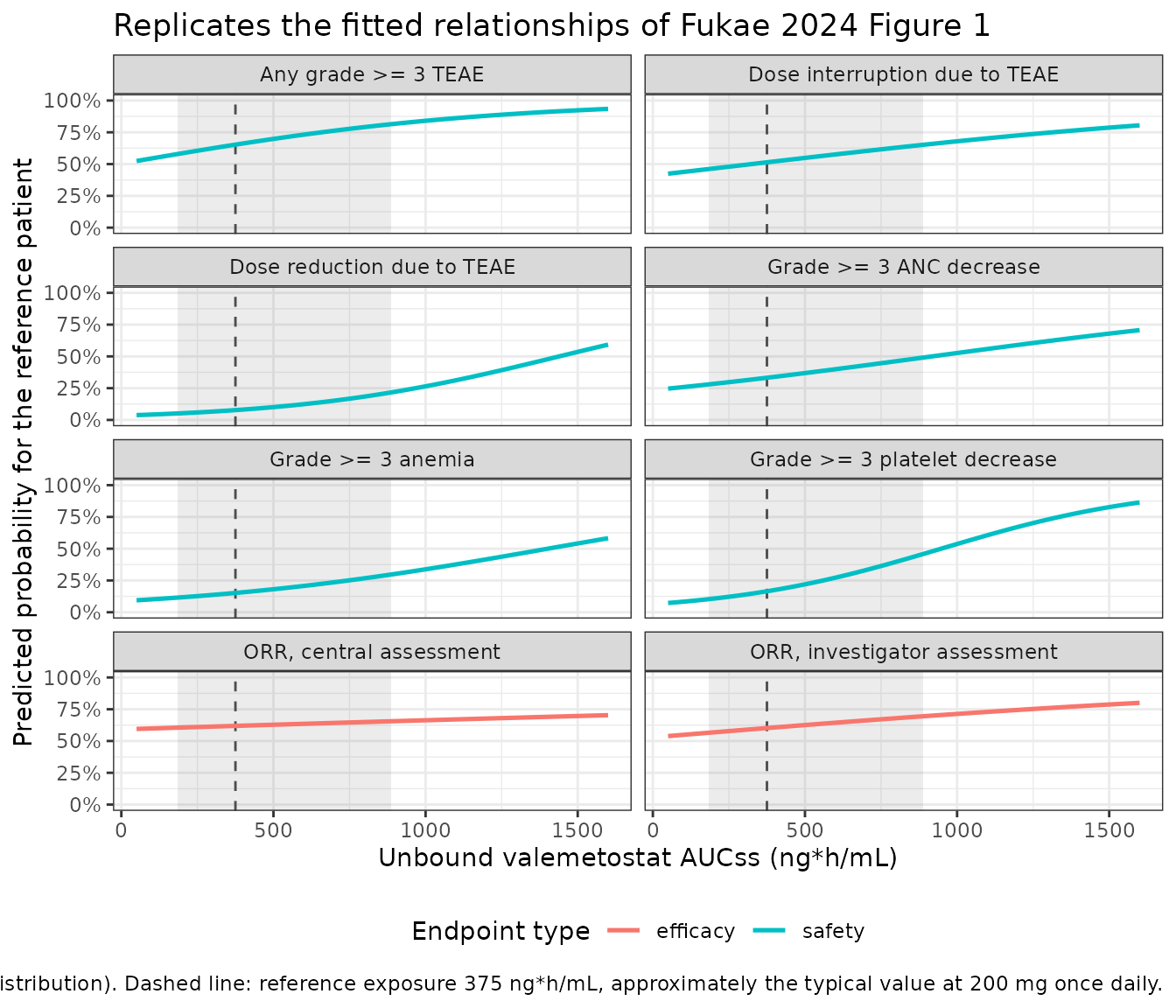
The qualitative claims of the paper’s Results and Discussion fall directly out of these curves, and the chunk below asserts them rather than leaving them to visual inspection: the exposure-efficacy relationships are shallow while the exposure-safety relationships are steeper, and the steepest of all is grade >= 3 platelet decrease.
slopes <- endpoints |>
  dplyr::rowwise() |>
  dplyr::mutate(
    or_per_250 = odds(solve_prob(mods[[model]], output, auc = 625)) /
                 odds(solve_prob(mods[[model]], output, auc = 375))
  ) |>
  dplyr::ungroup()

eff <- slopes |> dplyr::filter(set == "efficacy")
saf <- slopes |> dplyr::filter(set == "safety")

stopifnot(
  # "A slightly positive relationship was observed between unbound exposure and
  # efficacy endpoints. A steeper relationship was observed in safety
  # endpoints, compared with efficacy." (Abstract)
  all(eff$or_per_250 > 1), all(saf$or_per_250 > 1),
  max(eff$or_per_250) < min(saf$or_per_250),
  # "the highest increase of odds of TEAEs (103%)" for grade >= 3 PLT decrease.
  slopes$endpoint[which.max(slopes$or_per_250)] == "Grade >= 3 platelet decrease"
)

slopes |>
  dplyr::arrange(or_per_250) |>
  dplyr::transmute(
    Endpoint = endpoint, `Type` = set,
    `Odds ratio per 250 ng*h/mL` = round(or_per_250, 3),
    `Change in odds` = sprintf("%+.0f%%", 100 * (or_per_250 - 1))
  ) |>
  knitr::kable(
    caption = paste(
      "Every exposure effect is positive; all six safety slopes exceed both",
      "efficacy slopes, and grade >= 3 platelet decrease is steepest, exactly",
      "as reported in the Fukae 2024 Abstract and Discussion."
    )
)| Endpoint | Type | Odds ratio per 250 ng*h/mL | Change in odds |
|---|---|---|---|
| ORR, central assessment | efficacy | 1.08 | +8% |
| ORR, investigator assessment | efficacy | 1.22 | +22% |
| Dose interruption due to TEAE | safety | 1.32 | +32% |
| Grade >= 3 ANC decrease | safety | 1.38 | +38% |
| Any grade >= 3 TEAE | safety | 1.51 | +51% |
| Grade >= 3 anemia | safety | 1.52 | +52% |
| Dose reduction due to TEAE | safety | 1.79 | +79% |
| Grade >= 3 platelet decrease | safety | 2.03 | +103% |
Subpopulation predictions (Figure 3 and Figure S7)
Fukae 2024 Figure 3 reports predicted ORR by subpopulation at 200 mg. The packaged models reproduce the direction and ordering of those subgroup contrasts. The comparison is deliberately made at the reference exposure with one covariate varied at a time, which is the contrast the model parameterizes; the paper’s own figure additionally integrates over the covariate distribution observed within each subgroup and over the posterior, so its point estimates are not expected to match exactly (see Assumptions and deviations).
subpops <- tibble::tribble(
  ~subgroup,                ~cov,          ~value,
  "ECOG PS 0 (reference)",  "ECOG_GE1",    0,
  "ECOG PS 1+",             "ECOG_GE1",    1,
  "Male (reference)",       "SEXF",        0,
  "Female",                 "SEXF",        1,
  "Age 65 y (reference)",   "AGE",         65,
  "Age 75 y",               "AGE",         75,
  "Japan (reference)",      "REGION_USA",  0,
  "United States",          "REGION_USA",  1
)

subpop_pred <- subpops |>
  tidyr::expand_grid(dplyr::select(endpoints, model, endpoint, output)) |>
  dplyr::rowwise() |>
  dplyr::mutate(
    prob = solve_prob(mods[[model]], output,
                      stats::setNames(list(value), cov), auc = 375)
  ) |>
  dplyr::ungroup()

# ECOG PS 1+ lowers the odds of response on both efficacy models (Figure 3
# shows 0.37 vs 0.62 central and 0.55 vs 0.61 investigator).
ecog <- subpop_pred |>
  dplyr::filter(cov == "ECOG_GE1", grepl("ORR", endpoint, fixed = TRUE)) |>
  dplyr::select(endpoint, subgroup, prob) |>
  tidyr::pivot_wider(names_from = subgroup, values_from = prob)

stopifnot(nrow(ecog) == 2L, all(ecog$`ECOG PS 1+` < ecog$`ECOG PS 0 (reference)`))

subpop_pred |>
  dplyr::filter(model == "Fukae_2024_valemetostat_orr_central") |>
  dplyr::transmute(Subgroup = subgroup,
                   `Predicted ORR (central)` = round(prob, 3)) |>
  knitr::kable(
    caption = paste(
      "Single-covariate contrasts at the reference exposure for the",
      "central-assessment ORR model. The ECOG PS ordering reproduces the",
      "Fukae 2024 Figure 3 contrast (1+ well below 0)."
    )
)| Subgroup | Predicted ORR (central) |
|---|---|
| ECOG PS 0 (reference) | 0.619 |
| ECOG PS 1+ | 0.380 |
| Male (reference) | 0.619 |
| Female | 0.612 |
| Age 65 y (reference) | 0.619 |
| Age 75 y | 0.613 |
| Japan (reference) | 0.619 |
| United States | 0.619 |
Region of practical equivalence
The paper’s dose justification rests on a region of practical equivalence. The Methods define its two limits with different criteria, and the difference matters for what these packaged point-estimate models can and cannot reproduce.
-
Lower limit (efficacy). The lowest exposure
ewithP(ORR | E = e, X) >= pifor a proportionpof patients, withpi = 30%(the response rate assumed in the J201 sample-size calculation) andp = 50%. The paper states the reduction explicitly: this “is therefore equivalent to the exposure providing an expected ORR of 30% in a typical patient”. That is exactly a reference-patient calculation, so it is reproducible here. -
Upper limit (safety). The highest exposure
ewithP_X(P(dose reduction | E = e, X) <= pi) >= p, withpi = 50%andp = 90%– “90% of patients receiving an initial dose that is likely (probability >50%) to be maintained”. This is a population criterion: it integrates over the covariate distributionXand the posterior, neither of which is packaged. The published value of 1255ng*h/mLis therefore not a typical-patient quantity and is not reproduced exactly below; what is checked instead is the direction it must lie in.
p_at <- function(model_suffix, auc) {
  row <- endpoints |> dplyr::filter(model == paste0("Fukae_2024_valemetostat_", model_suffix))
  solve_prob(mods[[row$model]], row$output, auc = auc)
}

# Typical-patient exposure at which P(dose reduction) crosses the pi = 50%
# acceptability threshold.
auc_red50 <- stats::uniroot(
  function(a) p_at("dose_reduction", a) - 0.50, interval = c(375, 5000)
)$root

orr_at_zero  <- p_at("orr_central", 0)
red_at_upper <- p_at("dose_reduction", 887)

stopifnot(
  # LOWER LIMIT. The typical patient's predicted ORR never falls to the 30%
  # threshold at any non-negative exposure, so the theoretical lower limit is
  # 0 -- exactly the published value ("a theoretical ROPE extending beyond the
  # observed exposure range, from 0 to 1255 ng*h/mL", Results).
  orr_at_zero > 0.30,
  # UPPER LIMIT. The published 1255 ng*h/mL is a 90%-of-patients criterion, so
  # it must be strictly MORE conservative than the typical-patient crossing:
  # the binding subject is a more susceptible one than the reference patient.
  p_at("dose_reduction", 1255) < 0.50,
  auc_red50 > 1255,
  # Across the whole modified ROPE the typical patient stays far below the
  # threshold, which is why the paper could truncate to the observed range
  # without giving up acceptable safety.
  red_at_upper < 0.50
)

tibble::tibble(
  Quantity = c(
    "Predicted ORR (central) at zero exposure",
    "Predicted ORR (central) at the reference exposure, 375 ng*h/mL",
    "P(dose reduction) at the modified-ROPE upper limit, 887 ng*h/mL",
    "P(dose reduction) at the published theoretical upper limit, 1255 ng*h/mL",
    "Typical-patient exposure at which P(dose reduction) reaches 50%"
  ),
  Value = c(
    sprintf("%.1f%%", 100 * orr_at_zero),
    sprintf("%.1f%%", 100 * p_at("orr_central", 375)),
    sprintf("%.1f%%", 100 * red_at_upper),
    sprintf("%.1f%%", 100 * p_at("dose_reduction", 1255)),
    sprintf("%.0f ng*h/mL", auc_red50)
  ),
  Criterion = c(
    "> 30% required; never breached, so the theoretical lower limit is 0",
    "-", "< 50% required", "< 50% required",
    "must exceed the published 1255 ng*h/mL population limit"
  )
) |>
  knitr::kable(
    caption = paste(
      "The typical-patient efficacy criterion reproduces the published",
      "theoretical ROPE lower limit of 0 exactly. The upper limit is a",
      "90%-of-patients criterion and so is bounded, not reproduced: the",
      "typical-patient 50% crossing lies above the published 1255 ng*h/mL,",
      "as a population criterion requires."
    )
)| Quantity | Value | Criterion |
|---|---|---|
| Predicted ORR (central) at zero exposure | 59.1% | > 30% required; never breached, so the theoretical lower limit is 0 |
| Predicted ORR (central) at the reference exposure, 375 ng*h/mL | 61.9% | - |
| P(dose reduction) at the modified-ROPE upper limit, 887 ng*h/mL | 21.7% | < 50% required |
| P(dose reduction) at the published theoretical upper limit, 1255 ng*h/mL | 39.4% | < 50% required |
| Typical-patient exposure at which P(dose reduction) reaches 50% | 1439 ng*h/mL | must exceed the published 1255 ng*h/mL population limit |
Assumptions and deviations
No NCA validation section. The standard
PKNCAcross-check does not apply to this paper: there is no PK model and no concentration-time profile anywhere in it. Exposure is a scalar per-subject input drawn from the companion population PK publication (doi:10.1002/psp4.13201). Running NCA here would only recover a number the user supplied. The structural identities in “Structural verification” above are the substantive check, and they are stronger than an NCA comparison would be – they audit every one of the 138 published estimates exactly rather than comparing summary statistics.Centring and scaling constants are inferred, not printed. Fukae 2024 states the convention (“approximate population median and standard deviation”) but never tabulates the constants. They are recovered from the reference-patient footnotes (centres) and the per-row increments the odds ratios are quoted per (scales), then corroborated against the Table 1 cohort medians and standard deviations, as shown above. The recovery is exact in the sense that it reproduces every published odds ratio, but a reader should know the constants are inferred rather than transcribed.
Baseline laboratory reference values come from the Results narrative. The Table 3 footnote lists the reference patient’s age, weight, hepatic function, LDH and exposure but omits hemoglobin, ANC and platelets. Those three (115 g/L, 3 x 10^9/L, 200 x 10^9/L) are stated in the Results text for each corresponding endpoint and are used as the centring constants.
The Methods covariate list is narrower than Table 3. For the exposure-safety analysis the Methods name only region, sex, race, hepatic impairment and NHL stage as categorical candidates plus the baseline laboratory values as continuous ones – yet Table 3 additionally reports age, LDH and weight effects for all six safety models. The packaged models follow Table 3, per the standing convention that the printed parameter table outranks a narrative summary.
NHL disease stage is documented but not encoded. Stage (I-III vs IV) is named in Methods as a candidate covariate for both the efficacy and safety analyses, but appears in neither Table 2 nor Table 3, so no point estimate is available. It is recorded in each model’s
covariatesDataExcludedrather than guessed at. Stage was missing for 23.5% of the safety cohort and 35.9% of the ATLL cohort, the likely reason it was dropped.Placeholder residual error. The source models use a Bernoulli likelihood and estimate no residual error and no between-subject random effect. rxode2 requires an observation declaration, so each model emits its deterministic probability with a
fixed(0.001)additive residual, following theOniki_2018_nafld_risk.Rprecedent. This does not perturb the predicted probability – theprob_*column read throughout this vignette is the individual prediction, not a residual-perturbed simulation. To sample binary outcomes, applyrbinom(n, 1, prob_*)to therxSolve()output.Uncertainty is not propagated. Only the posterior medians are packaged. The published 95% credible intervals are wide – several exceed three orders of magnitude on the odds scale (the Black-race slope effects, where n = 6) – and every parameter’s interval is recorded in the source-trace comment beside its
ini()value, but the packaged models are point-estimate models. Any use that needs uncertainty must return to the paper’s posterior.The ROPE upper limit is bounded, not reproduced. The published theoretical ROPE is 0 to 1255 ngh/mL. The lower limit is a typical-patient criterion and is reproduced exactly above (the predicted ORR never falls to the 30% threshold, so the limit is 0). The upper limit is a population* criterion – the highest exposure at which 90% of patients still have below a 50% probability of dose reduction – and evaluating it requires the joint covariate distribution and the posterior, neither of which is packaged. The vignette therefore checks the inequality the criterion implies (the typical-patient 50% crossing must lie above 1255 ng*h/mL) rather than asserting the published number.
Subpopulation predictions are single-covariate contrasts. Figure 3 and Figure S7 of the paper integrate over the covariate distribution observed within each subgroup and over 1000 posterior draws. The vignette instead varies one covariate at a time at the reference exposure, so the ordering and direction reproduce but the point estimates are not expected to match the figure exactly.
Three new canonical covariate columns.
PLT(platelet count, general scope),AUCU_VALE(unbound valemetostat steady-state AUC) andREGION_USA(United States enrollment indicator) were registered ininst/references/covariate-columns.mdalongside this extraction.REGION_USAwas registered rather than reusingREGION_JAPANwith inverted coefficients because Fukae 2024’s reference category is Japan, so everyini()value reads straight off the published table without sign inversion. Eightprob_<endpoint>PD-output names were registered ininst/references/compartment-names.md, following the family shape founded byprob_rocand extended byprob_scc.