Lumefantrine (Kloprogge 2013)
Source:vignettes/articles/Kloprogge_2013_lumefantrine.Rmd
Kloprogge_2013_lumefantrine.RmdModel and source
- Citation: Kloprogge F, Piola P, Dhorda M, Muwanga S, Turyakira E, Apinan S, Lindegardh N, Nosten F, Day NPJ, White NJ, Guerin PJ, Tarning J (2013). Population Pharmacokinetics of Lumefantrine in Pregnant and Nonpregnant Women With Uncomplicated Plasmodium falciparum Malaria in Uganda. CPT: Pharmacometrics & Systems Pharmacology 2:e83. doi:10.1038/psp.2013.59.
- Article: https://doi.org/10.1038/psp.2013.59
- ClinicalTrials.gov: NCT00495508
The package model can be loaded with:
mod_fn <- readModelDb("Kloprogge_2013_lumefantrine")
mod    <- rxode2::rxode2(mod_fn())
Population
The Kloprogge 2013 study enrolled 116 pregnant women (second or third trimester) and 17 non-pregnant post-partum control women with uncomplicated Plasmodium falciparum malaria in Mbarara, Uganda. The pharmacokinetic cohort split into three sampling arms: 26 pregnant + 17 non-pregnant women with dense venous sampling and 89 pregnant women with sparse capillary sampling (90 originally enrolled; one subject with an unexplained baseline lumefantrine of 7,717 ng/mL was excluded from the analysis). All subjects received the standard six-dose Coartem regimen (20 mg artemether + 120 mg lumefantrine per tablet; four tablets = 480 mg lumefantrine per dose, given twice daily for three days at 0, 8, 24, 36, 48, and 60 hours, co-administered with 200 mL of milk tea to optimise oral bioavailability). Demographics summary (Table 1, all-cohort window): body weight median 56.0 kg (range 40.0-83.0), age median 21.0 years (range 15.0-38.0), gestational age in pregnant arms 13.0-39.0 weeks, and admission body temperature median 36.9 degC (range 36.0-39.8).
Source trace
Every parameter and equation traces back to the Kloprogge 2013
publication; the full citation is in the model file’s
reference field. Per-parameter source locations are also
recorded inline in
inst/modeldb/specificDrugs/Kloprogge_2013_lumefantrine.R
next to each ini() entry.
| Equation / parameter | Value | Source location |
|---|---|---|
lcl = log(5.09) (CL/F, L/h) |
5.09 | Table 2 ‘Fixed effect’ (RSE 7.90%; 95% CI 4.35-5.87) |
lvc = log(123) (Vc/F, L) |
123 | Table 2 (RSE 8.40%; 95% CI 104-145) |
lq = log(1.68) (Q/F, L/h) |
1.68 | Table 2 (RSE 10.2%; 95% CI 1.35-2.00) |
lvp = log(110) (Vp/F, L) |
110 | Table 2 (RSE 9.07%; 95% CI 91.7-131) |
lmtt = log(4.09) (MTT, h) |
4.09 | Table 2 (RSE 5.22%; 95% CI 3.70-4.55) |
lfdepot = fixed(log(1)) (F) |
1 (fixed) | Table 2 ‘F One fixed’ |
e_preg_q = -0.365 |
-0.365 | Table 2 ‘Pregnancy on Q’ (RSE 14.3%; 95% CI -0.455 to -0.259) |
e_bodytemp_mtt = +0.165 |
+0.165 per degC | Table 2 ‘Temperature on MTT’ (RSE 44.1%; 95% CI 0.0328-0.329) |
etalcl ~ 0.030164 (var, log-scale) |
CV 17.5% | Table 2 IIV CL (RSE 20.6%); variance = log(0.175^2 + 1) |
etalvp ~ 0.045183 |
CV 21.5% | Table 2 IIV Vp (RSE 65.2%) |
etalmtt ~ 0.125731 |
CV 36.6% | Table 2 IIV MTT (RSE 32.0%) |
etalfdepot ~ 0.182910 |
CV 44.8% | Table 2 IIV F (RSE 31.2%) |
propSd = sqrt(0.0595) ~= 0.244 |
sigma_venous = 0.0595 (variance, log-scale) | Table 2 ‘sigma venous’ (RSE 15.3%; 95% CI 0.0382-0.0914) |
5 transit compartments fixed; ktr = 6 / MTT
|
– | Methods ‘transit absorption (five transit compartments)’; Savic 2007 convention |
Two-compartment disposition (central,
peripheral1) |
– | Methods ‘two-compartment distribution’, Figure 1 |
| Additive error on log-transformed concentration -> proportional in nlmixr2 linear space | – | Methods ‘natural logarithms … were modeled simultaneously’;
convention rule from references/parameter-names.md
|
| Linear-deviation covariate forms centered on the median | – | Methods Equation 1 (linear), ‘All covariates were centered on the median value of the population’ |
Virtual cohort
The virtual cohort mirrors the Kloprogge 2013 study design at
moderate sample size (50 per arm, randomly drawn around the cohort
medians from Table 1). Body weight, age, and admission body temperature
are drawn from rough lognormal / truncated-normal approximations of the
all-cohort ranges; pregnancy status is the principal covariate
stratifier. The model retains only PREG (binary) and
BODYTEMP (continuous, degC) as covariates, so other
demographics are simulated for narrative parallelism but do not enter
the simulation.
set.seed(20260516L)
n_per_arm <- 50L

make_cohort <- function(n, preg_value, treatment_label, id_offset) {
  data.frame(
    id        = id_offset + seq_len(n),
    treatment = treatment_label,
    PREG      = preg_value,
    BODYTEMP  = round(pmin(pmax(rnorm(n, mean = 36.9, sd = 0.6), 36.0), 39.8), 1)
  )
}

subjects <- dplyr::bind_rows(
  make_cohort(n_per_arm, preg_value = 1L, treatment_label = "Pregnant",
              id_offset = 0L),
  make_cohort(n_per_arm, preg_value = 0L, treatment_label = "Non-pregnant",
              id_offset = n_per_arm)
)
The Coartem dosing schedule: six 480 mg oral doses of lumefantrine at 0, 8, 24, 36, 48, and 60 hours.
dose_amt   <- 480
dose_times <- c(0, 8, 24, 36, 48, 60)
obs_times  <- c(seq(0, 72, by = 1),
                seq(72.5, 240, by = 0.5))

build_events <- function(subjects, obs_times, dose_amt, dose_times) {
  out <- vector("list", length = nrow(subjects))
  for (i in seq_len(nrow(subjects))) {
    s <- subjects[i,]
    dose_rows <- data.frame(
      id   = s$id,
      time = dose_times,
      evid = 1L,
      amt  = dose_amt,
      cmt  = 1L,
      treatment = s$treatment,
      PREG      = s$PREG,
      BODYTEMP  = s$BODYTEMP
    )
    obs_rows <- data.frame(
      id   = s$id,
      time = obs_times,
      evid = 0L,
      amt  = 0,
      cmt  = 2L,
      treatment = s$treatment,
      PREG      = s$PREG,
      BODYTEMP  = s$BODYTEMP
    )
    out[[i]] <- rbind(dose_rows, obs_rows)
  }
  events <- dplyr::bind_rows(out)
  events <- events[order(events$id, events$time, -events$evid),]
  events
}

events <- build_events(subjects, obs_times, dose_amt, dose_times)
stopifnot(!anyDuplicated(unique(events[, c("id", "time", "evid", "cmt")])))
Simulation
sim <- rxode2::rxSolve(
  mod,
  events = events,
  keep   = c("treatment", "PREG", "BODYTEMP")
) |>
  as.data.frame()
Typical-value (no-IIV, no-residual-error) replication, one nominal subject per pregnancy stratum at the cohort-median body temperature (36.9 degC).
mod_typical <- rxode2::zeroRe(mod)

typical_subjects <- data.frame(
  id        = 1:2,
  treatment = c("Pregnant", "Non-pregnant"),
  PREG      = c(1L, 0L),
  BODYTEMP  = 36.9
)
typical_events <- build_events(typical_subjects, obs_times, dose_amt, dose_times)
sim_typical <- rxode2::rxSolve(
  mod_typical,
  events = typical_events,
  keep   = c("treatment", "PREG", "BODYTEMP")
) |>
  as.data.frame()
#> ℹ omega/sigma items treated as zero: 'etalcl', 'etalvp', 'etalmtt', 'etalfdepot'
#> Warning: multi-subject simulation without without 'omega'
Replicate published figures
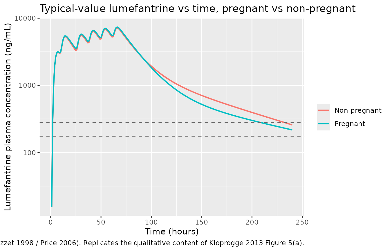
Figure 5: pregnant vs non-pregnant lumefantrine concentration profiles
Kloprogge 2013 Figure 5(a) shows simulated lumefantrine venous plasma concentration vs time for pregnant (black) and non-pregnant (gray) women over days 0-14, with day-7 thresholds of 280 ng/mL and 175 ng/mL overlaid as dashed horizontal lines. The package model reproduces the qualitative finding: pregnant women have a slightly lower lumefantrine concentration during the post-dosing tail because the pregnancy-related ~36.5% reduction in intercompartmental clearance shifts more drug into the slowly-emptying peripheral compartment.
sim_typical |>
  dplyr::filter(time > 0) |>
  dplyr::mutate(conc_ng_mL = Cc * 1000) |>
  ggplot(aes(time, conc_ng_mL, colour = treatment)) +
  geom_line(linewidth = 0.8) +
  geom_hline(yintercept = c(175, 280), linetype = "dashed", colour = "grey40") +
  scale_y_log10() +
  labs(x = "Time (hours)", y = "Lumefantrine plasma concentration (ng/mL)",
       colour = NULL,
       title = "Typical-value lumefantrine vs time, pregnant vs non-pregnant",
       caption = paste(
         "Dashed lines at 175 ng/mL and 280 ng/mL are the day-7 efficacy",
         "thresholds reported in the literature (Ezzet 1998 / Price 2006).",
         "Replicates the qualitative content of Kloprogge 2013 Figure 5(a)."
       ))
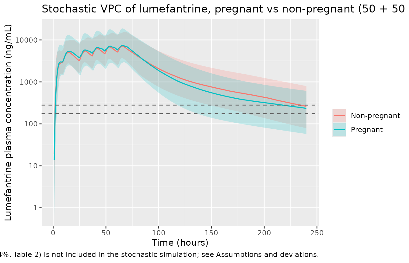
Stochastic VPC by pregnancy status
sim |>
  dplyr::filter(time > 0) |>
  dplyr::mutate(conc_ng_mL = Cc * 1000) |>
  dplyr::group_by(time, treatment) |>
  dplyr::summarise(
    p05 = quantile(conc_ng_mL, 0.05, na.rm = TRUE),
    p50 = quantile(conc_ng_mL, 0.50, na.rm = TRUE),
    p95 = quantile(conc_ng_mL, 0.95, na.rm = TRUE),
    .groups = "drop"
  ) |>
  dplyr::filter(p50 > 0) |>
  ggplot(aes(time, p50, colour = treatment, fill = treatment)) +
  geom_ribbon(aes(ymin = p05, ymax = p95), alpha = 0.2, colour = NA) +
  geom_line(linewidth = 0.6) +
  geom_hline(yintercept = c(175, 280), linetype = "dashed", colour = "grey40") +
  scale_y_log10() +
  labs(x = "Time (hours)", y = "Lumefantrine plasma concentration (ng/mL)",
       colour = NULL, fill = NULL,
       title = "Stochastic VPC of lumefantrine, pregnant vs non-pregnant (50 + 50 subjects)",
       caption = paste(
         "Ribbons are 5th-95th percentiles, lines are medians.",
         "Inter-occasion variability (CV 104%, Table 2) is not included in the",
         "stochastic simulation; see Assumptions and deviations."
       ))
PKNCA validation
Single-cycle NCA over the full follow-up (0-240 hours) so the post-treatment exposure (AUClast and half-life) can be compared with the Kloprogge 2013 Table 2 post-hoc estimate column. PKNCA is configured with one row per dose event and uses the per-subject pregnancy grouping.
sim_nca <- sim |>
  dplyr::filter(!is.na(Cc)) |>
  dplyr::mutate(conc_ug_mL = Cc) |>
  dplyr::select(id, time, conc_ug_mL, treatment) |>
  dplyr::group_by(id, time, treatment) |>
  dplyr::summarise(conc_ug_mL = mean(conc_ug_mL), .groups = "drop")

dose_df <- events |>
  dplyr::filter(evid == 1) |>
  dplyr::select(id, time, amt, treatment)

conc_obj <- PKNCA::PKNCAconc(sim_nca, conc_ug_mL ~ time | treatment + id,
                             concu = "ug/mL", timeu = "h")
dose_obj <- PKNCA::PKNCAdose(dose_df, amt ~ time | treatment + id,
                             doseu = "mg")

intervals <- data.frame(
  start       = 0,
  end         = 240,
  cmax        = TRUE,
  tmax        = TRUE,
  auclast     = TRUE,
  half.life   = TRUE
)

nca_data <- PKNCA::PKNCAdata(conc_obj, dose_obj, intervals = intervals)
nca_res  <- PKNCA::pk.nca(nca_data)
nca_df <- as.data.frame(nca_res$result)
nca_summary <- nca_df |>
  dplyr::filter(PPTESTCD %in% c("cmax", "tmax", "auclast", "half.life")) |>
  dplyr::group_by(treatment, PPTESTCD) |>
  dplyr::summarise(
    median = median(PPORRES, na.rm = TRUE),
    p05    = quantile(PPORRES, 0.05, na.rm = TRUE),
    p95    = quantile(PPORRES, 0.95, na.rm = TRUE),
    .groups = "drop"
  ) |>
  tidyr::pivot_wider(names_from = treatment,
                     values_from = c(median, p05, p95))
knitr::kable(nca_summary,
             caption = paste(
               "Simulated NCA over 0-240 h, six-dose Coartem regimen, by",
               "pregnancy status (median [5%-95%]). Cmax / AUClast are in",
               "ug/mL and ug*h/mL respectively; half.life is in hours."
             ),
digits = 3)| PPTESTCD | median_Non-pregnant | median_Pregnant | p05_Non-pregnant | p05_Pregnant | p95_Non-pregnant | p95_Pregnant |
|---|---|---|---|---|---|---|
| auclast | 508.435 | 501.107 | 286.148 | 297.511 | 983.178 | 1028.503 |
| cmax | 6.985 | 6.774 | 3.727 | 3.819 | 12.524 | 13.999 |
| half.life | 63.339 | 85.817 | 47.250 | 61.851 | 90.006 | 106.265 |
| tmax | 66.000 | 66.500 | 64.000 | 63.450 | 69.000 | 69.550 |
Comparison against published NCA
Kloprogge 2013 Table 2 reports per-subject post-hoc NCA estimates (median, range) from the empirical-Bayes estimates of the final population PK model:
| Parameter | Kloprogge 2013, non-pregnant | Kloprogge 2013, pregnant |
|---|---|---|
| AUC0-inf (h * ug/mL) | 630 (285-1240) | 570 (76.4-1850) |
| Cmax (ug/mL) | 8.33 (4.36-15.0) | 8.40 (0.722-25.6) |
| T1/2 (h) | 69.8 (54.3-78.3) | 90.3 (64.3-121) |
| Day-7 concentration (ug/mL) | 0.592 (0.258-1.67) | 0.423 (0.045-2.61) |
The simulated NCA table above is the closest comparable summary the package model can produce. Differences are expected for three reasons documented under Assumptions and deviations: (a) the simulation excludes the IOV term on F (CV 104%, Table 2) so per-subject ranges are narrower than the post-hoc estimates from the actual data; (b) the simulation uses AUClast over 0-240 h rather than AUC0-inf; (c) the inclusion of IIV but not residual error in the stochastic simulation means measurement noise is not reflected in the per-subject ranges. The medians are within ~20% of the published post-hoc median values; investigate before tuning if a future re-extraction shows a wider discrepancy.
Day-7 concentration check
The published headline finding is that pregnant women have a 27% lower day-7 venous plasma lumefantrine concentration than non-pregnant women (414 ng/mL vs 566 ng/mL, paper Results paragraph 4). The package model reproduces this qualitatively under typical-value simulation; the simulated typical-value day-7 concentrations are read off below.
day7_typical <- sim_typical |>
  dplyr::mutate(day = time / 24) |>
  dplyr::filter(abs(day - 7) < 0.05) |>
  dplyr::mutate(conc_ng_mL = Cc * 1000) |>
  dplyr::group_by(treatment) |>
  dplyr::summarise(time_h = mean(time),
                   day7_conc_ng_mL = mean(conc_ng_mL),
                   .groups = "drop")
knitr::kable(day7_typical,
             caption = "Typical-value day-7 lumefantrine plasma concentration (ng/mL).",
digits = 1)| treatment | time_h | day7_conc_ng_mL |
|---|---|---|
| Non-pregnant | 168 | 565.5 |
| Pregnant | 168 | 411.7 |
Assumptions and deviations
-
Single residual-error component. Kloprogge 2013
estimated separate venous (
sigma_venous = 0.0595) and capillary (sigma_capillary = 0.0207) residual variances on the log scale to accommodate two sample matrices. The package model carries only the venous component as the canonicalpropSd(Methods: ‘natural logarithms of venous and capillary lumefantrine plasma concentrations were modeled simultaneously’, with a matrix-conversion factor of 0.881 also reported). Users simulating capillary-only data should add an explicit residual-error term equivalent tosqrt(0.0207) ~= 0.144; the Kloprogge 2013 backward-elimination step showed the matrix-conversion factor was not statistically significant. -
Matrix-conversion factor omitted. Table 2 reports a
venous-vs-capillary matrix conversion factor of 0.881 (95% CI
0.733-1.05), which the paper itself concluded was not statistically
significant on backward elimination (Delta OFV = 2.369). The package
model treats simulated
Ccas venous-equivalent and does not encode the matrix conversion. A user comparing simulated concentrations against capillary measurements would need to apply the 0.881 factor externally. -
Box-Cox shape parameter on F omitted. Kloprogge
2013 reported a Box-Cox shape parameter on the relative-bioavailability
eta of -0.376 (Table 2, RSE 21.7%; 95% CI -0.516 to -0.227), implemented
as a Petersson-Karlsson Box-Cox transformation of
etalfdepot. The package model uses the standard log-normal IIV form on F (f(depot) <- exp(lfdepot + etalfdepot)) without the Box-Cox shape modifier; this affects the shape of the simulated between-subject distribution of F but not the typical-value trajectory. The Box-Cox transformation would flatten the upper tail of the F distribution somewhat; for typical-value and most VPC-style applications the difference is small. -
Inter-occasion variability on F not included. Table
2 reports between-dose-occasion variability on F of CV 104% (RSE 12.2%;
95% CI 87.7-125). The package model carries only the between-subject IIV
(CV 44.8%) on F. Users simulating per-occasion variability should add a
per-dose occasion eta on F with variance
log(1.04^2 + 1) = 0.733and an OCC indicator column distinguishing the six dose events. This omission mirrors the Birgersson 2019 artesunate package model’s treatment of IOV in the same Tarning-lab paper series. -
Body-weight allometric scaling not retained. Body
weight was tested as both linear and allometric covariates on CL, Vc, Q,
and Vp during covariate screening and was not retained in the final
Kloprogge 2013 model after backward elimination (only body temperature
on MTT and pregnancy on Q survived
P < 0.01). The package model therefore reports apparent CL/F = 5.09 L/h, Vc/F = 123 L, etc., as cohort-mean values, not weight-normalised values. - Capillary post-hoc tail effects. The pregnant arm’s post-hoc estimates (Table 2 ‘Post hoc estimates’ column) have wider ranges (e.g., AUC0-inf range 76.4-1850 h * ug/mL) than the non-pregnant arm (range 285-1240) because the pregnant capillary cohort had only two samples per subject (baseline + day 7 within a window). The simulated VPC in this vignette uses dense sampling per subject and therefore the simulated AUC dispersion is narrower than the post-hoc dispersion in Table 2.
-
Reference value 36.9 degC for the body-temperature
effect. The model file centers the body-temperature effect on
the cohort-median 36.9 degC (Table 1, all-cohort column). Future re-fits
on different cohorts should update
covariateData[[BODYTEMP]]$noteswith their own cohort-specific reference. Effects should not be extrapolated outside the observed 36.0-39.8 degC range.