Model and source
- Citation: Alli A, Paruk F, Roger C, Lipman J, Calleemalay D, Wallis SC, Scribante J, Richards GA, Roberts JA, Ballotta A. Peri-operative pharmacokinetics of cefazolin prophylaxis during valve replacement surgery. PLoS One. 2023;18(9):e0291425. doi:10.1371/journal.pone.0291425
- Description: Three-compartment joint total/unbound population PK model for intravenous cefazolin surgical prophylaxis in adults undergoing elective cardiac valve replacement with cardiopulmonary bypass (Alli 2023). The dose enters a central compartment whose concentration is the TOTAL plasma cefazolin; it exchanges first-order with a peripheral compartment and with a separate unbound-drug compartment (volume Vt) whose concentration is the UNBOUND plasma cefazolin. The return rate constant from the unbound compartment to the central (total) compartment is the protein-binding term PB = (ktc * Bmax + NS) * (ALB / 40), so higher serum albumin pulls drug back into the total pool. Clearance acts on the central compartment and scales inversely with serum creatinine, CL = TVCL * (90 / SeCr). Estimated with the Pmetrics non-parametric adaptive grid (NPAG); the non-parametric distribution is approximated here by log-normal IIV from the reported CV%.
- Article (open access): https://doi.org/10.1371/journal.pone.0291425
Alli and colleagues measured total and unbound plasma cefazolin in adults receiving 2 g cefazolin prophylaxis for elective cardiac valve replacement on cardiopulmonary bypass (CPB), fitted a joint total/unbound population PK model in Pmetrics (NPAG), and used it to estimate the probability of target attainment (PTA) of 100% fT>MIC over the first 4 hours of surgery.
The structure (Figure 2 of the paper) has three compartments:
- a central (“dosing”) compartment of volume Vc whose
concentration is the total plasma cefazolin; clearance
acts here and is scaled by serum creatinine,
CL = TVCL * (90 / SeCr); - a peripheral compartment exchanging with central through kcp / kpc;
- an unbound-drug compartment of volume Vt whose
concentration is the unbound plasma cefazolin. Drug
moves into it from central at rate kct and returns at the albumin-scaled
protein-binding rate constant
PB = (ktc * Bmax + NS) * (ALB / 40).
Population
Sixteen adults (8 women, 8 men; age 18-59 years, mean 44; weight 51-97 kg, mean 75.1) undergoing CPB for elective valve replacement at Charlotte Maxeke Johannesburg Academic Hospital, South Africa (Table 1 of the paper). Mean serum creatinine was 76.7 umol/L (range 42-102), mean serum albumin 41.6 g/L (range 33-47) and mean CPB duration 165 min. Each patient received 2 g cefazolin IV 30 minutes before incision, re-dosed with 2 g at 4 hours if surgery was ongoing. The analysis used 195 total and 64 unbound concentrations.
The same information is available programmatically:
str(readModelDb("Alli_2023_cefazolin")()$population)
#> List of 13
#>  $ species       : chr "human"
#>  $ n_subjects    : int 16
#>  $ n_studies     : int 1
#>  $ n_samples     : chr "195 total and 64 unbound plasma cefazolin concentrations"
#>  $ age_range     : chr "18-59 years (mean 44.0, SD 12.0)"
#>  $ weight_range  : chr "51-97 kg (mean 75.1, SD 15.6)"
#>  $ sex_female_pct: num 50
#>  $ disease_state : chr "Adults (18-60 years eligible) undergoing cardiopulmonary bypass (CPB) for elective cardiac valve replacement, r"| __truncated__
#>  $ renal_function: chr "Serum creatinine mean 76.7 umol/L (SD 18.6, range 42-102); Cockcroft-Gault creatinine clearance mean 81.5 mL/mi"| __truncated__
#>  $ albumin       : chr "Serum albumin mean 41.6 g/L (SD 4.57, range 33-47)."
#>  $ dose_range    : chr "2 g cefazolin IV (Figure 2: 1-min bolus infusion) 30 min before skin incision, re-dosed 2 g after 4 h if surgery was ongoing."
#>  $ regions       : chr "South Africa (Charlotte Maxeke Johannesburg Academic Hospital)"
#>  $ notes         : chr "Demographics from Alli 2023 Table 1. Prospective convenience-sampled PK study; plasma sampled pre-dose and 2-30"| __truncated__
Source trace
| Equation / parameter | Value | Source location |
|---|---|---|
lcl (CL at SeCr 90 umol/L) |
log(3.23) L/h | Table 2, Cl mean (CV 36.06%) |
lvc (Vc, total) |
log(3.38) L | Table 2, Vc mean (CV 21.59%) |
lvp2 (Vt, unbound compartment) |
log(6.08) L | Table 2, Vt mean (CV 33.42%) |
lk12 (kcp) |
log(5.92) 1/h | Table 2, kcp mean (CV 65.58%) |
lk21 (kpc) |
log(2.24) 1/h | Table 2, kpc mean (CV 51.81%) |
lk13 (kct) |
log(144.27) 1/h | Table 2, kct mean (CV 10.17%) |
lk31 (ktc) |
log(195.91) 1/h | Table 2, ktc mean (CV 12.94%) |
lbmax (Bmax) |
log(1.01) g/L | Table 2, Bmax mean (CV 45.23%) |
lkns (NS) |
log(15.14) | Table 2, NS mean (CV 24.79%) |
IIV (eta*) |
omega^2 = log(CV^2 + 1) | Table 2, CV% column |
addSd, propSd (total) |
1.0 mg/L, 0.1 | Results, assay error C0 and C1 for plasma data |
addSd_Cu, propSd_Cu (unbound) |
0.1 mg/L, 0.1 | Results, assay error C0 and C1 for unbound data |
cl = TVCL * (90 / CREAT) |
n/a | Results, ‘The final clearance model’ |
kpb = (k31 * bmax + kns) * (ALB / 40) |
n/a | Results, ‘The protein binding was described as follows’ |
| Three-compartment ODE structure | n/a | Results text and Figure 2 |
Cc = central / vc,
Cu = peripheral2 / vp2
|
n/a | Figure 2 volumes; Results (Vc central volume, Vt volume of the unbound compartment) |
Virtual cohort
Observed data are not public. The virtual cohort draws serum creatinine and albumin from normal distributions with the Table 1 means and SDs, truncated to the observed ranges. Subjects receive 2 g over 1 minute (Figure 2: ‘1 min bolus intravenous infusion’) at 0 and 4 hours and are sampled at the paper’s schedule (2-300 minutes).
set.seed(20230920)
rxode2::rxSetSeed(20230920)

n_sub <- 200
rtnorm <- function(n, mean, sd, lo, hi) {
  pmin(pmax(rnorm(n, mean, sd), lo), hi)
}
cohort <- tibble(
  id = seq_len(n_sub),
  CREAT = rtnorm(n_sub, 76.7, 18.6, 42, 102),
  ALB = rtnorm(n_sub, 41.6, 4.57, 33, 47)
)

# Paper sampling schedule (minutes after the first dose), converted to hours.
obs_min <- c(0, 2, 5, 10, 30, 60, 90, 120, 150, 180, 210, 240, 270, 300)

# Builds a dosing + observation event table. Doses are 1-minute infusions into
# `central`; observation rows carry dvid = 1 because the model declares two
# endpoints (Cc, Cu) -- both come back as columns on every observation row.
make_events <- function(cov, dose_times, dose_amts, obs_times) {
  doses <- tidyr::expand_grid(id = cov$id, k = seq_along(dose_times)) |>
    mutate(time = dose_times[k], amt = dose_amts[k], rate = amt * 60,
           evid = 1L, cmt = "central", dvid = NA_integer_) |>
    select(-k)
  obs <- tidyr::expand_grid(id = cov$id, time = obs_times) |>
    mutate(amt = 0, rate = 0, evid = 0L, cmt = "central", dvid = 1L)
  bind_rows(doses, obs) |>
    left_join(cov, by = "id") |>
    arrange(id, time, desc(evid))
}

events <- make_events(cohort, c(0, 4), c(2000, 2000), obs_min / 60)
stopifnot(!anyDuplicated(unique(events[, c("id", "time", "evid")])))
Simulation
mod <- readModelDb("Alli_2023_cefazolin")
sim <- rxode2::rxSolve(mod, events = events, returnType = "data.frame") |>
  filter(!is.na(Cc))
#> ℹ parameter labels from comments will be replaced by 'label()'

# Typical patient at the cohort-mean covariates.
typ_events <- make_events(tibble(id = 1L, CREAT = 76.7, ALB = 41.6),
                          c(0, 4), c(2000, 2000), obs_min / 60)
sim_typ <- rxode2::rxSolve(rxode2::zeroRe(mod), events = typ_events,
                           returnType = "data.frame")
#> ℹ parameter labels from comments will be replaced by 'label()'
#> ℹ omega/sigma items treated as zero: 'etalcl', 'etalvc', 'etalvp2', 'etalk12', 'etalk21', 'etalk13', 'etalk31', 'etalbmax', 'etalkns'
Replicate published figures
Figure 1 – mean total and unbound concentrations
Figure 1 of the paper plots the observed mean (SD) total and unbound concentrations at each sampling time. The means below were read from that figure by the maintainers (approximately +/- 5 mg/L).
fig1 <- tibble(
  minute = obs_min[-1],
  total_obs = c(317, 260, 210, 159, 112, 80, 72, 66, 61, 56, 50, 169, 138),
  unbound_obs = c(145, 119, 97, 73, 52, 38, 35, 32, 29, 27, 24, 78, 64)
)

typ_cmp <- sim_typ |>
  mutate(minute = round(time * 60)) |>
  filter(minute > 0) |>
  select(minute, total_typ = Cc, unbound_typ = Cu) |>
  left_join(fig1, by = "minute") |>
  mutate(
    total_pct = 100 * (total_typ - total_obs) / total_obs,
    unbound_pct = 100 * (unbound_typ - unbound_obs) / unbound_obs
  )

typ_cmp |>
  mutate(across(where(is.numeric), \(x) round(x, 1))) |>
  rename(
    "Minute" = minute,
    "Total, typical (mg/L)" = total_typ,
    "Total, Fig 1 mean (mg/L)" = total_obs,
    "Total diff (%)" = total_pct,
    "Unbound, typical (mg/L)" = unbound_typ,
    "Unbound, Fig 1 mean (mg/L)" = unbound_obs,
    "Unbound diff (%)" = unbound_pct
  ) |>
knitr::kable(caption = "Typical-patient prediction (SeCr 76.7 umol/L, ALB 41.6 g/L) against the Figure 1 observed means.")| Minute | Total, typical (mg/L) | Unbound, typical (mg/L) | Total, Fig 1 mean (mg/L) | Unbound, Fig 1 mean (mg/L) | Total diff (%) | Unbound diff (%) |
|---|---|---|---|---|---|---|
| 2 | 318.6 | 117.4 | 317 | 145 | 0.5 | -19.0 |
| 5 | 263.6 | 97.0 | 260 | 119 | 1.4 | -18.5 |
| 10 | 201.9 | 74.1 | 210 | 97 | -3.9 | -23.7 |
| 30 | 116.5 | 42.3 | 159 | 73 | -26.7 | -42.0 |
| 60 | 93.9 | 34.0 | 112 | 52 | -16.1 | -34.5 |
| 90 | 82.8 | 30.0 | 80 | 38 | 3.5 | -21.1 |
| 120 | 73.3 | 26.6 | 72 | 35 | 1.8 | -24.1 |
| 150 | 64.9 | 23.5 | 66 | 32 | -1.7 | -26.5 |
| 180 | 57.5 | 20.8 | 61 | 29 | -5.8 | -28.2 |
| 210 | 50.9 | 18.4 | 56 | 27 | -9.1 | -31.7 |
| 240 | 45.1 | 16.3 | 50 | 24 | -9.8 | -31.9 |
| 270 | 156.4 | 56.8 | 169 | 78 | -7.4 | -27.2 |
| 300 | 129.3 | 46.9 | 138 | 64 | -6.3 | -26.8 |
# Deterministic (typical-value) comparison, so a tight bound is safe. The total
# concentration is the primary endpoint (195 samples) and the model reproduces
# its mean profile: a mis-transcribed CL, Vc or binding constant moves the whole
# profile by tens of percent.
stopifnot(abs(median(typ_cmp$total_pct)) < 10)
# Unbound fraction implied by the binding structure at the typical covariates.
# The model's Cu / Cc settles near 0.36; the observed means in Figure 1 sit
# nearer 0.45-0.5 (see Assumptions and deviations).
fu_typ <- with(sim_typ[sim_typ$time > 1, ], median(Cu / Cc))
stopifnot(fu_typ > 0.3, fu_typ < 0.45)
fu_typ
#> [1] 0.3624384
# Replicates Figure 1 of Alli 2023 (observed means) with a VPC overlay.
vpc <- sim |>
  select(id, time, Total = Cc, Unbound = Cu) |>
  pivot_longer(c(Total, Unbound), names_to = "analyte", values_to = "conc") |>
  group_by(time, analyte) |>
  summarise(
    Q05 = quantile(conc, 0.05), Q50 = quantile(conc, 0.50),
    Q95 = quantile(conc, 0.95), mean = mean(conc), .groups = "drop"
  )
obs_long <- fig1 |>
  pivot_longer(c(total_obs, unbound_obs), names_to = "analyte", values_to = "conc") |>
  mutate(analyte = ifelse(analyte == "total_obs", "Total", "Unbound"),
         time = minute / 60)

ggplot(vpc, aes(time * 60, Q50, colour = analyte, fill = analyte)) +
  geom_ribbon(aes(ymin = Q05, ymax = Q95), alpha = 0.2, colour = NA) +
  geom_line() +
  geom_point(data = obs_long, aes(y = conc), shape = 21, size = 2) +
  labs(x = "Time after first dose (min)", y = "Cefazolin (mg/L)",
       colour = NULL, fill = NULL,
       caption = paste("Lines/ribbons: simulated median and 90% interval (n = 200).",
                       "Points: observed means read from Figure 1 of Alli 2023."))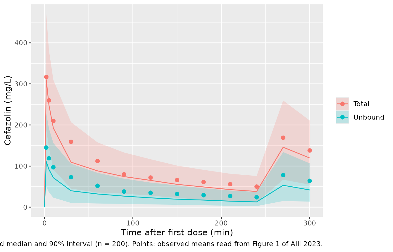
Figure 3 – probability of target attainment
The paper’s PTA simulations require the unbound
concentration to exceed the MIC for 100% of the first 4 hours of
surgery, and (Methods) compute the unbound concentration as a
fixed 26% of the total – the ‘worst case’ unbound
fraction the authors measured at 120 minutes – rather than from the
model’s unbound compartment. The replication below does the same: the
target is 0.26 * Cc >= MIC at every time point from the
end of the first infusion to 4 hours. Doses inside the 4-hour window are
those of each regimen (a 4-hourly regimen contributes only its first
dose).
pta_grid <- sort(unique(c(seq(1 / 60, 4, by = 2 / 60), 2 - 1e-3, 4)))
mic_grid <- 2^(-4:6)

pta_scenarios <- tribble(
  ~panel, ~label, ~creat, ~alb, ~t2, ~d1, ~d2,
  "a", "1g4h", 50, 35, NA, 1000, NA,
  "a", "2g4h", 50, 35, NA, 2000, NA,
  "a", "3g4h", 50, 35, NA, 3000, NA,
  "a", "1g2h", 50, 35, 2, 1000, 1000,
  "a", "2g2h", 50, 35, 2, 2000, 2000,
  "a", "2g/1g 2h", 50, 35, 2, 2000, 1000,
  "a", "3g/1.5g 2h", 50, 35, 2, 3000, 1500,
  "b", "Cr50", 50, 35, NA, 2000, NA,
  "b", "Cr75", 75, 35, NA, 2000, NA,
  "b", "Cr100", 100, 35, NA, 2000, NA,
  "c", "Alb30", 75, 30, NA, 3000, NA,
  "c", "Alb35", 75, 35, NA, 3000, NA,
  "c", "Alb40", 75, 40, NA, 3000, NA
) |>
  mutate(scenario = row_number())

pta_events <- bind_rows(lapply(seq_len(nrow(pta_scenarios)), function(i) {
  s <- pta_scenarios[i, ]
  times <- if (is.na(s$t2)) 0 else c(0, s$t2)
  amts <- if (is.na(s$t2)) s$d1 else c(s$d1, s$d2)
  cov <- tibble(id = (i - 1L) * n_sub + seq_len(n_sub),
                CREAT = s$creat, ALB = s$alb, scenario = i)
  make_events(cov, times, amts, pta_grid)
}))
stopifnot(!anyDuplicated(unique(pta_events[, c("id", "time", "evid")])))

pta_sim <- rxode2::rxSolve(mod, events = pta_events, keep = "scenario",
                           returnType = "data.frame")

trough_free <- pta_sim |>
  filter(time >= 1 / 60) |>
  group_by(scenario, id) |>
  summarise(min_free = min(0.26 * Cc), .groups = "drop")

pta <- tidyr::expand_grid(scenario = pta_scenarios$scenario, mic = mic_grid) |>
  left_join(trough_free, by = "scenario", relationship = "many-to-many") |>
  group_by(scenario, mic) |>
  summarise(pta = mean(min_free >= mic), .groups = "drop") |>
  left_join(pta_scenarios |> select(scenario, panel, label), by = "scenario")
# Replicates Figure 3a-c of Alli 2023.
panel_titles <- c(a = "(a) regimens, SeCr 50, ALB 35",
                  b = "(b) 2 g 4-hourly, ALB 35",
                  c = "(c) 3 g 4-hourly, SeCr 75")
ggplot(pta, aes(mic, pta, colour = label)) +
  geom_line() +
  geom_point(size = 1) +
  scale_x_log10(breaks = mic_grid, labels = format(mic_grid, drop0trailing = TRUE)) +
  facet_wrap(~panel, ncol = 2, labeller = labeller(panel = panel_titles)) +
  labs(x = "MIC (mg/L)", y = "PTA (100% fT>MIC, 0-4 h)", colour = NULL,
       caption = "Simulated with 0.26 x total concentration as unbound; n = 200 per curve.")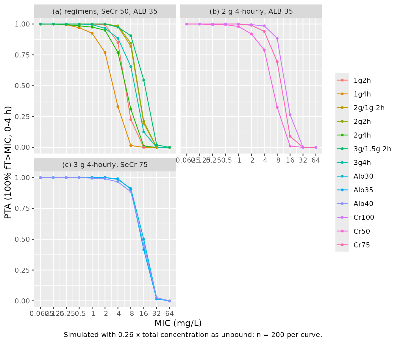
The legible curves of Figure 3 were read by the maintainers at the plotted MIC values (approximately +/- 0.03). The comparison uses the MIC at which PTA crosses 50% (interpolated on the log2 MIC scale), which is insensitive to which subjects land in the tails.
pub_pta <- tribble(
  ~label, ~mic, ~pta_pub,
  "1g4h", 1, 0.95, "1g4h", 2, 0.80, "1g4h", 4, 0.38, "1g4h", 8, 0.04,
  "2g4h", 2, 0.96, "2g4h", 4, 0.80, "2g4h", 8, 0.39, "2g4h", 16, 0.03,
  "3g4h", 4, 0.92, "3g4h", 8, 0.64, "3g4h", 16, 0.20, "3g4h", 32, 0,
  "Cr75", 4, 0.97, "Cr75", 8, 0.79, "Cr75", 16, 0.16, "Cr75", 32, 0,
  "Cr100", 8, 0.95, "Cr100", 16, 0.37, "Cr100", 32, 0, "Cr100", 64, 0,
  "Alb30", 4, 0.92, "Alb30", 8, 0.65, "Alb30", 16, 0.20, "Alb30", 32, 0,
  "Alb35", 4, 0.99, "Alb35", 8, 0.95, "Alb35", 16, 0.55, "Alb35", 32, 0.03,
  "Alb40", 4, 0.99, "Alb40", 8, 0.95, "Alb40", 16, 0.55, "Alb40", 32, 0.03
)

# log2 MIC at which a decreasing PTA curve crosses 0.5.
mic50 <- function(mic, p) {
  o <- order(mic)
  mic <- mic[o]
  p <- p[o]
  i <- which(p >= 0.5 & c(p[-1], 0) < 0.5)[1]
  if (i == length(p)) return(log2(mic[i]))
  log2(mic[i]) + (p[i] - 0.5) / (p[i] - p[i + 1]) * (log2(mic[i + 1]) - log2(mic[i]))
}

sim_mic50 <- pta |>
  filter(label %in% unique(pub_pta$label)) |>
  group_by(label) |>
  summarise(sim = mic50(mic, pta), .groups = "drop")
pub_mic50 <- pub_pta |>
  group_by(label) |>
  summarise(pub = mic50(mic, pta_pub), .groups = "drop")
mic50_cmp <- left_join(pub_mic50, sim_mic50, by = "label") |>
  mutate(diff_dilutions = sim - pub,
         label = factor(label, levels = unique(pub_pta$label))) |>
  arrange(label)

mic50_cmp |>
  mutate(across(where(is.numeric), \(x) round(2^x, 2), .names = "{.col}_mgL"),
         diff_dilutions = round(diff_dilutions, 2)) |>
  select(label, pub_mgL, sim_mgL, diff_dilutions) |>
  rename(
    "Curve" = label,
    "MIC50, Figure 3 (mg/L)" = pub_mgL,
    "MIC50, simulated (mg/L)" = sim_mgL,
    "Difference (doubling dilutions)" = diff_dilutions
  ) |>
knitr::kable(caption = "MIC at which PTA crosses 50%: Figure 3 versus simulation.")| Curve | MIC50, Figure 3 (mg/L) | MIC50, simulated (mg/L) | Difference (doubling dilutions) |
|---|---|---|---|
| 1g4h | 3.28 | 3.06 | -0.10 |
| 2g4h | 6.64 | 6.01 | -0.14 |
| 3g4h | 9.97 | 9.80 | -0.03 |
| Cr75 | 11.01 | 10.00 | -0.14 |
| Cr100 | 13.70 | 12.30 | -0.15 |
| Alb30 | 10.08 | 16.00 | 0.67 |
| Alb35 | 17.10 | 14.19 | -0.27 |
| Alb40 | 17.10 | 14.88 | -0.20 |
# Regimen, renal-function and albumin 35 / 40 g/L curves must land within one
# doubling dilution of the published curve. The albumin 30 g/L curve of
# Figure 3c is a known deviation and is not gated -- see Assumptions and
# deviations.
gated <- mic50_cmp |> filter(label != "Alb30")
stopifnot(
  abs(median(gated$diff_dilutions)) < 0.5,
  all(abs(gated$diff_dilutions) < 1)
)
PKNCA validation
The paper reports no NCA table. NCA over the first dosing interval (0-4 h) is computed per analyte on the paper’s sampling schedule, so the simulated Cmax is the 2-minute concentration – the same quantity as the first plotted point of Figure 1, which serves as the reference.
nca_conc <- sim |>
  filter(time <= 4) |>
  select(id, time, Total = Cc, Unbound = Cu) |>
  pivot_longer(c(Total, Unbound), names_to = "analyte", values_to = "Cc") |>
  filter(!is.na(Cc))
# Pre-dose rows are present at time 0 (Cc = 0); guard anyway.
nca_conc <- bind_rows(
  nca_conc,
  nca_conc |> distinct(id, analyte) |> mutate(time = 0, Cc = 0)
) |>
  distinct(id, analyte, time, .keep_all = TRUE) |>
  arrange(analyte, id, time)

nca_dose <- events |>
  filter(evid == 1, time == 0) |>
  select(id, time, amt) |>
  tidyr::expand_grid(analyte = c("Total", "Unbound"))

conc_obj <- PKNCA::PKNCAconc(nca_conc, Cc ~ time | analyte + id)
dose_obj <- PKNCA::PKNCAdose(nca_dose, amt ~ time | analyte + id)
intervals <- data.frame(start = 0, end = 4, cmax = TRUE, tmax = TRUE,
                        auclast = TRUE)
nca_res <- PKNCA::pk.nca(PKNCA::PKNCAdata(conc_obj, dose_obj, intervals = intervals))
summary(nca_res)
#>  start end analyte   N    auclast       cmax                    tmax
#>      0   4   Total 200 301 [38.9] 304 [29.0] 0.0333 [0.0333, 0.0333]
#>      0   4 Unbound 200 108 [74.4] 111 [50.1] 0.0333 [0.0333, 0.0333]
#>
#> Caption: auclast, cmax: geometric mean and geometric coefficient of variation; tmax: median and range; N: number of subjects
Comparison against published values
published <- tibble::tribble(
  ~analyte, ~cmax,
  "Total", 317,
  "Unbound", 145
)
cmp <- nlmixr2lib::ncaComparisonTable(
  simulated = nca_res,
  reference = published,
  by = "analyte",
  params = "cmax",
  units = c(cmax = "mg/L"),
  tolerance_pct = 20
)
knitr::kable(cmp, caption = "Simulated median Cmax (2 min) against the Figure 1 observed mean at 2 min. * differs by >20%.")| NCA parameter | analyte | Reference | Simulated | % diff |
|---|---|---|---|---|
| Cmax (mg/L) | Total | 317 | 310 | -2.2% |
| Cmax (mg/L) | Unbound | 145 | 111 | -23.5%* |
The total Cmax agrees closely. The unbound Cmax is lower than observed, for the reason given below.
Assumptions and deviations
- Typical values are the Table 2 means. Pmetrics NPAG returns a discrete non-parametric population distribution, summarised in Table 2 by mean, SD, CV%, variance and median. The mean is used as the typical value (it is the figure the Results text quotes), and each CV% becomes a log-normal IIV variance, omega^2 = log(CV^2 + 1), with no covariances. This is a parametric approximation of the non-parametric distribution.
-
Residual-error multiplier. Pmetrics multiplies the
assay-error polynomial
SD = C0 + C1 * obsby an estimated noise factor gamma; the paper prints C0 and C1 but not gamma. The polynomial is used unscaled (gamma = 1) as acombined1additive-plus-proportional error. -
Reading of the binding term. The Results define
PB = (ktc * Bmax + NS) * (ALB / 40)as ‘the rate constant for protein binding from unbound to total drug’, and Figure 2 draws Bmax and NS acting on the unbound-to-central arrow. PB is therefore the rate constant of that arrow, replacing ktc there; kct is the central-to-unbound rate constant. Bmax is tabulated in g/L and NS without a unit; both are used as dimensionless multipliers exactly as the equation is printed. This reading reproduces the Figure 1 total profile (median difference -5.8%). The alternative (PB as the central-to-unbound constant) was checked by the maintainers and fits the total peak markedly worse (about 250 versus 317 mg/L at 2 minutes). - Unbound concentrations are under-predicted. At the cohort-mean covariates the model’s unbound-to-total ratio settles at about 0.36, whereas the Figure 1 means imply about 0.45-0.5, so the typical unbound profile runs roughly 20-40% below the observed means. The paper reports no individual or population predictions for unbound concentrations beyond the S1 goodness-of-fit scatter, so the gap cannot be traced further; it is not tuned away. Note that the paper itself did not use the model’s unbound output for its PTA work but a fixed 26% unbound fraction.
- Covariate references. The clearance equation normalises SeCr to 90 umol/L and the binding term normalises albumin to 40 g/L, both described as ‘the population mean value’, whereas Table 1 reports means of 76.7 umol/L and 41.6 g/L. The printed equation values are used.
- The 30 g/L albumin curve of Figure 3c is not reproduced. In the model, albumin barely moves the total-concentration trough, so with the paper’s fixed 26% unbound fraction the three albumin curves nearly coincide. The 35 and 40 g/L curves match Figure 3c, but the published 30 g/L curve sits about two-thirds of a doubling dilution to the left. That curve is numerically identical to the 3 g 4-hourly curve of Figure 3a (SeCr 50 umol/L), which the simulation does reproduce, so the panel may carry a labelling issue. It is shown but not gated.
- Figure 3d (surgery duration) is not replicated. Its 5- and 6-hour curves fall below the 4-hour curve under a 4-hourly regimen, which implies the re-dose was not given at 4 hours in those simulations; the timing used is not stated.
- Window of the target. PTA is evaluated from the end of the first 1-minute infusion to 4 hours after the first dose; the paper says ‘the first 4 hours of surgery’ without stating whether the 30-minute pre-incision interval is included.
- Virtual cohort. Creatinine and albumin are drawn from truncated normals with the Table 1 means, SDs and ranges; the paper’s covariate distribution is otherwise unreported. Fixed covariates (SeCr, ALB) are used for the PTA scenarios, as in the paper.
- Digitised values. The Figure 1 means and Figure 3 PTA values were read by the maintainers from the published figures.
- No correction notice for this article was found on Europe PMC (checked 2026-10-27).