Temocillin PK/PD against Escherichia coli (van Os 2024)
Source:vignettes/articles/vanOs_2024_temocillin.Rmd
vanOs_2024_temocillin.RmdModel and source
van Os and colleagues combined static time-kill (STK) experiments and a hollow-fibre infection model (HFIM) to build a semi-mechanistic PK/PD model of temocillin activity against four Escherichia coli strains, then coupled that PD model to a published population PK model of temocillin in critically ill patients in order to compare dosing regimens.
The paper fitted the PD model separately for each of the four strains (Table 3 reports four independent columns of estimates with their own relative standard errors), so the extraction is four model files that share one structure, plus this single vignette.
strainModels <- c(
  "ATCC 25922" = "vanOs_2024_temocillin_atcc25922",
  "ISOL MIC16" = "vanOs_2024_temocillin_isolmic16",
  "ISOL MIC8"  = "vanOs_2024_temocillin_isolmic8",
  "ISOL MIC4"  = "vanOs_2024_temocillin_isolmic4"
)
strainMIC <- c("ATCC 25922" = 16, "ISOL MIC16" = 16, "ISOL MIC8" = 8, "ISOL MIC4" = 4)

mod1 <- readModelDb(strainModels[["ATCC 25922"]])- Citation: van Os W, Nussbaumer-Proll A, Pham AD, Wijnant GJ, Ngougni Pokem P, Van Bambeke F, van Hasselt JGC, Zeitlinger M. Pharmacokinetic/pharmacodynamic model-based optimization of temocillin dosing strategies for the treatment of systemic infections. J Antimicrob Chemother. 2024;79(10):2484-2492. doi:10.1093/jac/dkae243. Structural equations: main-text Equations 1-3. Pharmacodynamic parameter estimates: main-text Table 3, column ATCC 25922. Strain characteristics: main-text Table 1. Population pharmacokinetic parameters: main-text Table 2, reproduced from Laterre PF, Wittebole X, Van de Velde S, Muller AE, Mouton JW, Carryn S, Tulkens PM, Dugernier T. Temocillin (6 g daily) in critically ill patients: continuous infusion versus three times daily administration. J Antimicrob Chemother. 2015;70(3):891-898. doi:10.1093/jac/dku465. Structure and coupling verified against the Supplementary data file NONMEM_code.txt.
- Article: https://doi.org/10.1093/jac/dkae243
- Supplementary data (includes the NONMEM simulation control stream
NONMEM_code.txt): https://doi.org/10.1093/jac/dkae243
Population
The pharmacodynamic layer is in vitro. Four E. coli strains were chosen to span the less susceptible end of the wild-type MIC distribution for the species (4-16 mg/L): the reference strain ATCC 25922 (MIC 16 mg/L) and three clinical isolates from the Vienna General Hospital – ISOL MIC16 (catheter urine, blaCTX-M-15 and blaOXA-1, MIC 16 mg/L), ISOL MIC8 (skin swab, MIC 8 mg/L) and ISOL MIC4 (rectal swab, blaTEM-1 and blaCTX-M-1, MIC 4 mg/L) (main-text Table 1). MICs were determined in triplicate by broth microdilution following CLSI guidelines.
STK experiments were run in triplicate in 5 mL cation-adjusted Mueller-Hinton broth at 37 degrees C, inoculated at 1.5e6 cfu/mL, over temocillin concentrations of 0.125-8x MIC plus a growth control, sampled over 24 h. The HFIM replicated the unbound plasma concentration-time profiles of four intravenous regimens over 72 h. Total counts were read on drug-free agar and the resistant subpopulation on agar containing 32 mg/L temocillin; the theoretical limit of detection was 50 cfu/mL and observations below it were handled with the M3 method.
The pharmacokinetic layer is not fitted in this
paper. It is the two-compartment population PK model of temocillin in
critically ill patients from Laterre et al. 2015 (n = 11), whose
parameter values this paper reproduces in its Table 2 and hard-codes in
the supplementary NONMEM control stream. All PK parameters and their
inter-individual variances are therefore encoded with
fixed().
The same information is available programmatically:
str(readModelDb(strainModels[["ATCC 25922"]])()$population, max.level = 1)
#> List of 9
#>  $ species         : chr "in vitro (Escherichia coli ATCC 25922); pharmacokinetics from critically ill adults"
#>  $ n_subjects      : int 1
#>  $ n_studies       : int 1
#>  $ strain          : chr "ATCC 25922 (reference strain; ESBL genes: none reported; temocillin MIC 16 mg/L, determined in triplicate by br"| __truncated__
#>  $ disease_state   : chr "Escherichia coli selected to span the less susceptible end of the wild-type MIC distribution for the species (4"| __truncated__
#>  $ model_system    : chr "Static time-kill (STK) experiments in 5 mL cation-adjusted Mueller-Hinton broth at 37 degrees C, in triplicate,"| __truncated__
#>  $ dose_range      : chr "HFIM regimens replicated over 72 h: 2 g q12h and 2 g q8h intermittent infusion, and 4 g/day and 6 g/day continu"| __truncated__
#>  $ initial_inoculum: chr "The published simulations set the total bacterial population at time zero to 1e6 cfu/mL and scaled each subpopu"| __truncated__
#>  $ notes           : chr "Estimated in NONMEM 7.4 with Laplacian estimation, PsN 5.3.0 and Pirana 21.11.1. The model was built in three s"| __truncated__
Source trace
Model equations
| Equation | Source location |
|---|---|
d/dt(bact_susceptible), sigmoidal Emax kill and
logistic growth |
Equation 1 (p. 2487) |
d/dt(bact_less_susceptible), sigmoidal Emax kill and
logistic growth |
Equation 2 (p. 2487) |
d/dt(bact_resistant), linear kill, growth capped on
S + LS
|
Equation 3 (p. 2487) |
Two-compartment plasma PK; Cu = central / vc * fu
drives all three effects |
Table 2; Supplementary NONMEM_code.txt $PK
/ $DES
|
Total count reported as log10(S + LS); resistant count
capped at the total |
Methods “PK/PD model”; Supplementary NONMEM_code.txt
$ERROR
|
| Rescaling of the fitted inocula to a 1e6 cfu/mL total at time zero | Methods “PK/PD simulations”; NONMEM_code.txt
THETA(1), THETA(6),
THETA(11)
|
Parameters
Every ini() entry carries an in-file comment naming its
source. The table below collects the values from all four strain models
in one place; the pharmacodynamic values are main-text Table 3 and the
pharmacokinetic values are main-text Table 2.
iniOf <- function(mn) {
  d <- rxode2::rxode(readModelDb(mn))$iniDf
  d <- d[!is.na(d$name), ]
  data.frame(Parameter = d$name, est = d$est, fixed = d$fix, stringsAsFactors = FALSE)
}
tr <- Reduce(
  function(a, b) dplyr::full_join(a, b, by = "Parameter"),
  Map(function(nm, mn) {
    x <- iniOf(mn)
    x$value <- ifelse(x$fixed, paste0(signif(x$est, 6), " (FIX)"), as.character(signif(x$est, 6)))
    stats::setNames(x[, c("Parameter", "value")], c("Parameter", nm))
  }, names(strainModels), strainModels)
)
#> ℹ parameter labels from comments will be replaced by 'label()'
#> ℹ parameter labels from comments will be replaced by 'label()'
#> ℹ parameter labels from comments will be replaced by 'label()'
#> ℹ parameter labels from comments will be replaced by 'label()'
tr$Source <- ifelse(
  grepl("^(lcl|lvc|lq|lvp|fu|etalcl|etalvc)$", tr$Parameter),
  "Table 2 (from Laterre et al. 2015)",
  ifelse(tr$Parameter == "log10cfu0_total", "Methods, PK/PD simulations", "Table 3")
)
knitr::kable(tr, caption = "Parameter values by strain, with source location. Log-scale PK parameters are shown on the log scale as stored in ini().")| Parameter | ATCC 25922 | ISOL MIC16 | ISOL MIC8 | ISOL MIC4 | Source |
|---|---|---|---|---|---|
| lcl | 1.30563 (FIX) | 1.30563 (FIX) | 1.30563 (FIX) | 1.30563 (FIX) | Table 2 (from Laterre et al. 2015) |
| lvc | 2.63906 (FIX) | 2.63906 (FIX) | 2.63906 (FIX) | 2.63906 (FIX) | Table 2 (from Laterre et al. 2015) |
| lq | 2.13417 (FIX) | 2.13417 (FIX) | 2.13417 (FIX) | 2.13417 (FIX) | Table 2 (from Laterre et al. 2015) |
| lvp | 3.07731 (FIX) | 3.07731 (FIX) | 3.07731 (FIX) | 3.07731 (FIX) | Table 2 (from Laterre et al. 2015) |
| fu | 0.41 (FIX) | 0.41 (FIX) | 0.41 (FIX) | 0.41 (FIX) | Table 2 (from Laterre et al. 2015) |
| kg_s | 1.29 | 1.39 | 1.51 | 1.47 | Table 3 |
| kg_ls | 0.797 | 0.795 | 0.72 | 0.796 | Table 3 |
| kg_res | 0.583 | 0.589 | 0.51 | 0.558 | Table 3 |
| log10bmax | 10 | 9.94 | 10.1 | 10.4 | Table 3 |
| emax_s | 2.06 | 2.38 | 2.86 | 2.38 | Table 3 |
| ec50_s | 3.56 | 8.31 | 3.75 | 1.57 | Table 3 |
| hill_s | 10 (FIX) | 2.45 | 3.51 | 2.73 | Table 3 |
| emax_ls | 0.777 | 1.09 | 1.01 | 0.843 | Table 3 |
| ec50_ls | 17.1 | 37 | 17.1 | 6.34 | Table 3 |
| hill_ls | 1.68 | 1 (FIX) | 1.79 | 10 (FIX) | Table 3 |
| klin_res | 0.00867 | 0.0094 | 0.0137 | 0.0421 | Table 3 |
| log10cfu0_s | 5.75 | 5.83 | 5.79 | 5.78 | Table 3 |
| log10cfu0_ls | 1.3 | 0.837 | 2.09 | 2.08 | Table 3 |
| log10cfu0_res | 0.237 | 0.528 | 0.156 | -0.271 | Table 3 |
| log10cfu0_total | 6 (FIX) | 6 (FIX) | 6 (FIX) | 6 (FIX) | Methods, PK/PD simulations |
| addSd_CFUtotal | 0.403 | 0.507 | 0.555 | 0.413 | Table 3 |
| addSd_CFUres | 0.614 | 0.711 | 0.655 | 0.638 | Table 3 |
| etalcl | 0.121864 (FIX) | 0.121864 (FIX) | 0.121864 (FIX) | 0.121864 (FIX) | Table 2 (from Laterre et al. 2015) |
| etalvc | 0.289979 (FIX) | 0.289979 (FIX) | 0.289979 (FIX) | 0.289979 (FIX) | Table 2 (from Laterre et al. 2015) |
Virtual cohort
Original observed data are not publicly available. The simulations below reproduce the paper’s Monte Carlo design: virtual critically ill patients carrying the Laterre inter-individual variability on clearance and central volume, with no residual variability, exactly as described in Methods (“PK/PD simulations”).
The paper simulated 1000 patients per regimen. This vignette uses 100 per arm across the 4 strains x 6 regimens grid to stay inside the library’s cohort cap and render budget; the consequence for three borderline cells is quantified in Assumptions and deviations.
set.seed(20240720)
nSub <- 100L

regimens <- c("2 g q12h II", "2 g q8h II", "4 g/day CI + 2 g LD",
              "6 g/day CI + 2 g LD", "8 g/day CI + 2 g LD", "12 g/day CI + 2 g LD")

# One subject's dosing records for a regimen. Doses are in mg and infusion
# rates in mg/h, matching the model's units metadata. Intermittent infusions
# run over 30 min (Methods, HFIM); continuous infusions are encoded as a single
# 72 h infusion at the daily rate, preceded by a 2 g loading dose.
doseRecords <- function(regimen, hours = 72) {
  ld <- as.data.frame(rxode2::et(amt = 2000, rate = 4000, cmt = "central"))
  ci <- function(gPerDay) {
    rt <- gPerDay * 1000 / 24
    as.data.frame(rxode2::et(amt = rt * hours, rate = rt, cmt = "central"))
  }
  ii <- function(interval) {
    as.data.frame(rxode2::et(amt = 2000, rate = 4000, ii = interval,
                             addl = ceiling(hours / interval) - 1, cmt = "central"))
  }
  switch(
    regimen,
    "2 g q12h II"          = ii(12),
    "2 g q8h II"           = ii(8),
    "4 g/day CI + 2 g LD"  = dplyr::bind_rows(ld, ci(4)),
    "6 g/day CI + 2 g LD"  = dplyr::bind_rows(ld, ci(6)),
    "8 g/day CI + 2 g LD"  = dplyr::bind_rows(ld, ci(8)),
    "12 g/day CI + 2 g LD" = dplyr::bind_rows(ld, ci(12))
  )
}

# CFUtotal and CFUres are DECLARED endpoints of these models (they appear in
# predDf), so observation rows must carry cmt = "CFUtotal" -- pointing them at
# an ODE state such as "central" is what fails here. See Assumptions.
makeCohort <- function(regimen, obsTimes, n, idOffset = 0L, hours = 72) {
  one <- dplyr::bind_rows(
    doseRecords(regimen, hours = hours),
    as.data.frame(rxode2::et(obsTimes, cmt = "CFUtotal"))
  )
  dplyr::bind_rows(lapply(seq_len(n), function(i) {
    dplyr::mutate(one, id = idOffset + i, regimen = regimen)
  }))
}

events <- dplyr::bind_rows(lapply(seq_along(regimens), function(k) {
  makeCohort(regimens[k], obsTimes = c(24, 72), n = nSub, idOffset = (k - 1L) * nSub)
}))
stopifnot(!anyDuplicated(unique(events[, c("id", "time", "evid")])))
stopifnot(dplyr::n_distinct(events$id) == nSub * length(regimens))
Simulation
The Laterre inter-individual variances are supplied explicitly to
rxSolve(); rxSolve otherwise reuses the
previous solve’s omega.
omegaPK <- lotri::lotri(etalcl ~ 0.1218636, etalvc ~ 0.2899794)

simStrain <- function(modelName, ev) {
  s <- rxode2::rxSolve(
    readModelDb(modelName), ev,
    omega = omegaPK, keep = "regimen",
    addDosing = FALSE, useLinCmt = FALSE,
    returnType = "data.frame"
  )
  stopifnot(dplyr::n_distinct(s$id) == dplyr::n_distinct(ev$id))
  s
}

simFig3 <- dplyr::bind_rows(lapply(names(strainModels), function(sn) {
  simStrain(strainModels[[sn]], events) |> dplyr::mutate(strain = sn)
}))
#> ℹ parameter labels from comments will be replaced by 'label()'
#> ℹ parameter labels from comments will be replaced by 'label()'
#> ℹ parameter labels from comments will be replaced by 'label()'
#> ℹ parameter labels from comments will be replaced by 'label()'
simFig3$strain <- factor(simFig3$strain, levels = names(strainModels))
simFig3$regimen <- factor(simFig3$regimen, levels = regimens)
Replicate published figures
Time course of the total and resistant populations
The paper’s full PK and PD time courses are Figure S4. This block shows the typical-value (zero random effects) trajectory for every strain and regimen, which is the deterministic backbone of the Monte Carlo simulations summarised in Figure 3.
tcTimes <- seq(0, 72, by = 0.5)
tcEvents <- dplyr::bind_rows(lapply(regimens, function(rg) {
  dplyr::bind_rows(doseRecords(rg), as.data.frame(rxode2::et(tcTimes, cmt = "CFUtotal"))) |>
    dplyr::mutate(id = 1L, regimen = rg)
}))

simTC <- dplyr::bind_rows(lapply(names(strainModels), function(sn) {
  m <- rxode2::zeroRe(readModelDb(strainModels[[sn]]))
  rxode2::rxSolve(m, tcEvents, omega = NA, keep = "regimen",
                  addDosing = FALSE, useLinCmt = FALSE,
                  returnType = "data.frame") |>
    dplyr::mutate(strain = sn)
}))
#> ℹ parameter labels from comments will be replaced by 'label()'
#> ℹ parameter labels from comments will be replaced by 'label()'
#> ℹ parameter labels from comments will be replaced by 'label()'
#> ℹ parameter labels from comments will be replaced by 'label()'
simTC$strain <- factor(simTC$strain, levels = names(strainModels))
simTC$regimen <- factor(simTC$regimen, levels = regimens)

simTC |>
  dplyr::select(time, strain, regimen, Total = CFUtotal, Resistant = CFUres) |>
  tidyr::pivot_longer(c(Total, Resistant), names_to = "Population", values_to = "logCfu") |>
  # The ODE is continuous, so a fully eradicated subpopulation keeps decaying
  # below any biologically meaningful count; clamp for display only.
  dplyr::mutate(logCfu = pmax(logCfu, -2)) |>
  ggplot(aes(time, logCfu, colour = Population)) +
  geom_hline(yintercept = 6, linetype = "dashed", colour = "grey40") +
  geom_line() +
  facet_grid(strain ~ regimen) +
  labs(x = "Time (h)", y = expression(log[10]~cfu/mL),
       title = "Typical-value bacterial time courses",
       caption = paste("Companion to Figure S4 of van Os 2024. Dashed line is the",
                       "initial total population (stasis level, 1e6 cfu/mL).")) +
  theme_bw() + theme(legend.position = "bottom")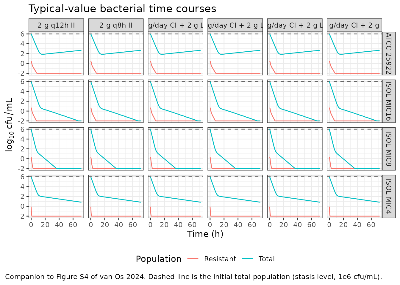
Figure 3 – predicted counts at 24 h and 72 h
fig3 <- simFig3 |>
  dplyr::filter(time %in% c(24, 72)) |>
  dplyr::select(id, time, strain, regimen, Total = CFUtotal, Resistant = CFUres) |>
  tidyr::pivot_longer(c(Total, Resistant), names_to = "Population", values_to = "logCfu") |>
  dplyr::mutate(logCfu = pmax(logCfu, -2),
                Timepoint = factor(paste0(time, " h"), levels = c("24 h", "72 h")))

ggplot(fig3, aes(regimen, logCfu, fill = Population)) +
  geom_hline(yintercept = c(4, 6), linetype = "dashed", colour = "grey40") +
  geom_boxplot(outlier.size = 0.4) +
  facet_grid(strain ~ Timepoint) +
  labs(x = NULL, y = expression(log[10]~cfu/mL),
       title = "Predicted bacterial counts at 24 h and 72 h",
       caption = paste("Replicates Figure 3 of van Os 2024 (unbound fraction 0.41).",
                       "Dashed lines are the initial total population (1e6 cfu/mL)",
                       "and a 2 log10 reduction.")) +
  theme_bw() +
  theme(axis.text.x = element_text(angle = 40, hjust = 1), legend.position = "bottom")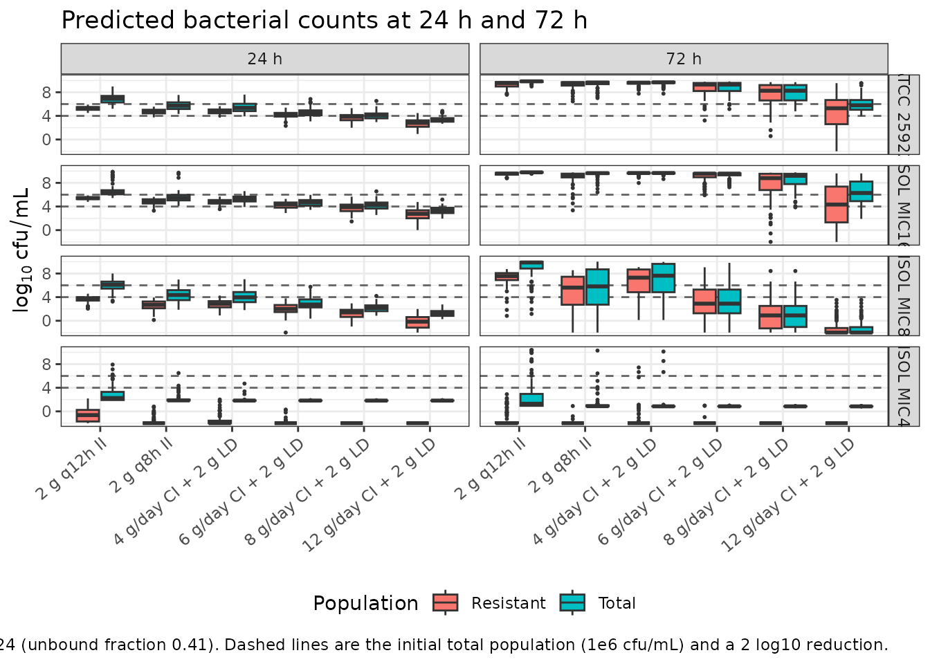
Quantitative check of the paper’s regimen claims
The Results section makes several sharp, falsifiable statements about the median predicted counts. Each is restated below as a test against the simulation.
med <- simFig3 |>
  dplyr::group_by(strain, regimen, time) |>
  dplyr::summarise(cfu = median(CFUtotal), .groups = "drop") |>
  tidyr::pivot_wider(names_from = time, values_from = cfu, names_prefix = "h")

knitr::kable(
  med |> dplyr::rename("Strain" = strain, "Regimen" = regimen,
                       "Median log10 cfu/mL at 24 h" = h24,
                       "Median log10 cfu/mL at 72 h" = h72),
  digits = 2,
  caption = "Median predicted total bacterial count. Stasis level is 6.00 log10 cfu/mL."
)| Strain | Regimen | Median log10 cfu/mL at 24 h | Median log10 cfu/mL at 72 h |
|---|---|---|---|
| ATCC 25922 | 2 g q12h II | 6.89 | 9.85 |
| ATCC 25922 | 2 g q8h II | 5.72 | 9.64 |
| ATCC 25922 | 4 g/day CI + 2 g LD | 5.36 | 9.68 |
| ATCC 25922 | 6 g/day CI + 2 g LD | 4.50 | 9.30 |
| ATCC 25922 | 8 g/day CI + 2 g LD | 4.11 | 8.26 |
| ATCC 25922 | 12 g/day CI + 2 g LD | 3.30 | 5.79 |
| ISOL MIC16 | 2 g q12h II | 6.30 | 9.79 |
| ISOL MIC16 | 2 g q8h II | 5.47 | 9.65 |
| ISOL MIC16 | 4 g/day CI + 2 g LD | 5.34 | 9.67 |
| ISOL MIC16 | 6 g/day CI + 2 g LD | 4.70 | 9.56 |
| ISOL MIC16 | 8 g/day CI + 2 g LD | 4.24 | 9.20 |
| ISOL MIC16 | 12 g/day CI + 2 g LD | 3.32 | 6.29 |
| ISOL MIC8 | 2 g q12h II | 6.09 | 9.87 |
| ISOL MIC8 | 2 g q8h II | 4.36 | 5.82 |
| ISOL MIC8 | 4 g/day CI + 2 g LD | 3.96 | 7.63 |
| ISOL MIC8 | 6 g/day CI + 2 g LD | 2.74 | 2.90 |
| ISOL MIC8 | 8 g/day CI + 2 g LD | 2.17 | 0.90 |
| ISOL MIC8 | 12 g/day CI + 2 g LD | 1.19 | -2.09 |
| ISOL MIC4 | 2 g q12h II | 2.26 | 1.29 |
| ISOL MIC4 | 2 g q8h II | 1.86 | 0.88 |
| ISOL MIC4 | 4 g/day CI + 2 g LD | 1.83 | 0.85 |
| ISOL MIC4 | 6 g/day CI + 2 g LD | 1.83 | 0.85 |
| ISOL MIC4 | 8 g/day CI + 2 g LD | 1.83 | 0.85 |
| ISOL MIC4 | 12 g/day CI + 2 g LD | 1.83 | 0.85 |
g <- function(st, rg, tp) med[[paste0("h", tp)]][med$strain == st & med$regimen == rg]
others <- function(st, rg, tp) med[[paste0("h", tp)]][med$strain == st & med$regimen != rg]

claims <- tibble::tibble(
  Claim = c(
    "ATCC 25922: 24 h median below stasis for every regimen except 2 g q12h",
    "ISOL MIC16: 24 h median below stasis for every regimen except 2 g q12h",
    "ATCC 25922: 72 h median reaches stasis only with the 12 g daily CI regimen",
    "ISOL MIC16: 72 h median reaches stasis only with the 12 g daily CI regimen",
    "ISOL MIC8: 24 h median below stasis for all simulated regimens",
    "ISOL MIC8: 72 h median stasis for 6 g daily regimens but not 4 g daily regimens",
    "ISOL MIC8: 2 log10 reduction at 72 h with 6 g/day CI and with 8 g/day",
    "ISOL MIC4: sustained killing (72 h median below stasis) for all regimens",
    "Continuous infusion beats intermittent infusion at 4 g/day (all strains, 72 h)",
    "Continuous infusion beats intermittent infusion at 6 g/day (all strains, 72 h)"
  ),
  Result = c(
    g("ATCC 25922", "2 g q12h II", 24) > 6 && all(others("ATCC 25922", "2 g q12h II", 24) < 6),
    g("ISOL MIC16", "2 g q12h II", 24) > 6 && all(others("ISOL MIC16", "2 g q12h II", 24) < 6),
    g("ATCC 25922", "12 g/day CI + 2 g LD", 72) < 6 &&
      all(others("ATCC 25922", "12 g/day CI + 2 g LD", 72) > 6),
    g("ISOL MIC16", "12 g/day CI + 2 g LD", 72) < 6 &&
      all(others("ISOL MIC16", "12 g/day CI + 2 g LD", 72) > 6),
    all(med$h24[med$strain == "ISOL MIC8"] < 6),
    g("ISOL MIC8", "6 g/day CI + 2 g LD", 72) < 6 && g("ISOL MIC8", "2 g q8h II", 72) < 6 &&
      g("ISOL MIC8", "4 g/day CI + 2 g LD", 72) > 6 && g("ISOL MIC8", "2 g q12h II", 72) > 6,
    g("ISOL MIC8", "6 g/day CI + 2 g LD", 72) < 4 && g("ISOL MIC8", "8 g/day CI + 2 g LD", 72) < 4,
    all(med$h72[med$strain == "ISOL MIC4"] < 6),
    all(vapply(names(strainModels), function(s)
      g(s, "4 g/day CI + 2 g LD", 72) < g(s, "2 g q12h II", 72), logical(1))),
    all(vapply(names(strainModels), function(s)
      g(s, "6 g/day CI + 2 g LD", 72) < g(s, "2 g q8h II", 72), logical(1)))
  )
) |>
  dplyr::mutate(Result = ifelse(Result, "reproduced", "see Assumptions"))

knitr::kable(claims, caption = "Published Results statements checked against the packaged models.")| Claim | Result |
|---|---|
| ATCC 25922: 24 h median below stasis for every regimen except 2 g q12h | reproduced |
| ISOL MIC16: 24 h median below stasis for every regimen except 2 g q12h | reproduced |
| ATCC 25922: 72 h median reaches stasis only with the 12 g daily CI regimen | reproduced |
| ISOL MIC16: 72 h median reaches stasis only with the 12 g daily CI regimen | see Assumptions |
| ISOL MIC8: 24 h median below stasis for all simulated regimens | see Assumptions |
| ISOL MIC8: 72 h median stasis for 6 g daily regimens but not 4 g daily regimens | reproduced |
| ISOL MIC8: 2 log10 reduction at 72 h with 6 g/day CI and with 8 g/day | reproduced |
| ISOL MIC4: sustained killing (72 h median below stasis) for all regimens | reproduced |
| Continuous infusion beats intermittent infusion at 4 g/day (all strains, 72 h) | reproduced |
| Continuous infusion beats intermittent infusion at 6 g/day (all strains, 72 h) | reproduced |
Structural checks against the supplementary control stream
The supplementary NONMEM_code.txt is a simulation
control stream for ATCC 25922. Three of its numbers can be checked
directly.
mz <- rxode2::zeroRe(readModelDb(strainModels[["ATCC 25922"]]))
#> ℹ parameter labels from comments will be replaced by 'label()'
t0 <- rxode2::rxSolve(mz, as.data.frame(rxode2::et(0, cmt = "CFUtotal")),
                      omega = NA, useLinCmt = FALSE, returnType = "data.frame")

# No-drug growth control: the total population must plateau at Bmax.
gc <- rxode2::rxSolve(mz, as.data.frame(rxode2::et(seq(0, 72, by = 1), cmt = "CFUtotal")),
                      omega = NA, useLinCmt = FALSE, returnType = "data.frame")

checks <- tibble::tibble(
  Quantity = c("Susceptible count at t = 0 (cfu/mL)",
               "Less susceptible count at t = 0 (cfu/mL)",
               "Resistant count at t = 0 (cfu/mL)",
               "Total count at t = 0 (log10 cfu/mL)",
               "Growth-control plateau at 72 h (log10 cfu/mL)"),
  Model = c(t0$bact_susceptible[1], t0$bact_less_susceptible[1], t0$bact_resistant[1],
            t0$CFUtotal[1], gc$CFUtotal[gc$time == 72]),
  Reference = c(1e6 - 10^1.55, 10^1.55, 10^0.487, 6, 10),
  Source = c("NONMEM_code.txt A_0(3), total 1e6 less the LS count",
             "NONMEM_code.txt A_0(4) = 10^THETA(6), THETA(6) = 1.55",
             "NONMEM_code.txt A_0(5) = 10^THETA(11), THETA(11) = 0.487",
             "Methods, PK/PD simulations: total set to 1e6 cfu/mL",
             "Table 3: Bmax,HFIM = 10.0 log10 cfu/mL")
)
knitr::kable(checks, digits = 4,
caption = "Model output versus the supplementary control stream and Table 3.")| Quantity | Model | Reference | Source |
|---|---|---|---|
| Susceptible count at t = 0 (cfu/mL) | 999964.5199 | 999964.5187 | NONMEM_code.txt A_0(3), total 1e6 less the LS count |
| Less susceptible count at t = 0 (cfu/mL) | 35.4801 | 35.4813 | NONMEM_code.txt A_0(4) = 10^THETA(6), THETA(6) = 1.55 |
| Resistant count at t = 0 (cfu/mL) | 3.0689 | 3.0690 | NONMEM_code.txt A_0(5) = 10^THETA(11), THETA(11) = 0.487 |
| Total count at t = 0 (log10 cfu/mL) | 6.0000 | 6.0000 | Methods, PK/PD simulations: total set to 1e6 cfu/mL |
| Growth-control plateau at 72 h (log10 cfu/mL) | 10.0000 | 10.0000 | Table 3: Bmax,HFIM = 10.0 log10 cfu/mL |
The scaling rule itself reproduces the control stream’s
$THETA block exactly: the Table 3 estimates for ATCC 25922
(5.75, 1.30 and 0.237 log10 cfu/mL) sum to a total of 5.750 log10
cfu/mL, so raising the total to 6 requires a shift of 0.25 log10 units,
giving 6, 1.55 and 0.487 – the values printed as THETA(1),
THETA(6) and THETA(11).
PKNCA validation
The pharmacodynamic layer is an in vitro bacterial count model for which NCA is not the relevant check (that layer is validated above against the control stream and Figure 3). The pharmacokinetic layer, however, is an ordinary two-compartment plasma model, and NCA gives an exact identity to test against: at steady state the AUC over one dosing interval must equal the dose divided by clearance. The PK is identical across the four strain models, so one model suffices.
The terminal half-life of the Laterre model is 7.89 h, so the 72 h
therapeutic window used above still carries about half a percent of
residual accumulation. The identity AUCtau = Dose / CL
holds only at true steady state, so this block dose for 144 h and takes
the interval starting at 120 h, on a 0.05 h grid fine enough that
trapezoidal error does not dominate.
set.seed(20240720)
nPK <- 200L
pkRegimens <- c("2 g q12h II", "2 g q8h II")
pkHours <- 144
ssStart <- 120

pkEvents <- dplyr::bind_rows(lapply(seq_along(pkRegimens), function(k) {
  makeCohort(pkRegimens[k], obsTimes = c(0, seq(ssStart, ssStart + 12, by = 0.05)),
             n = nPK, idOffset = (k - 1L) * nPK, hours = pkHours)
}))
stopifnot(dplyr::n_distinct(pkEvents$id) == nPK * length(pkRegimens))

simPK <- simStrain(strainModels[["ATCC 25922"]], pkEvents)
simPK$regimen <- factor(simPK$regimen, levels = pkRegimens)
simNca <- simPK |>
  dplyr::filter(!is.na(Cc)) |>
  dplyr::select(id, time, Cc, regimen)

# Guarantee a time-zero record per (id, regimen); pre-dose concentration is 0.
simNca <- dplyr::bind_rows(
  simNca,
  simNca |> dplyr::distinct(id, regimen) |> dplyr::mutate(time = 0, Cc = 0)
) |>
  dplyr::distinct(id, regimen, time, .keep_all = TRUE) |>
  dplyr::arrange(id, regimen, time)

doseDf <- pkEvents |>
  dplyr::filter(evid != 0) |>
  dplyr::select(id, time, amt, regimen)

concObj <- PKNCA::PKNCAconc(as.data.frame(simNca), Cc ~ time | regimen + id,
                            concu = "mg/L", timeu = "h")
doseObj <- PKNCA::PKNCAdose(as.data.frame(doseDf), amt ~ time | regimen + id,
                            doseu = "mg")

# One steady-state dosing interval per regimen, beginning at ssStart.
intervals <- data.frame(
  start   = c(ssStart, ssStart),
  end     = ssStart + c(12, 8),
  cmax    = TRUE,
  cmin    = TRUE,
  tmax    = TRUE,
  auclast = TRUE,
  cav     = TRUE
)

ncaRes <- PKNCA::pk.nca(PKNCA::PKNCAdata(concObj, doseObj, intervals = intervals))
ncaSum <- as.data.frame(ncaRes$result) |>
  dplyr::filter(!is.na(PPORRES)) |>
  dplyr::group_by(regimen, start, end, PPTESTCD) |>
  dplyr::summarise(median = median(PPORRES), .groups = "drop")
tau <- c("2 g q12h II" = 12, "2 g q8h II" = 8)

# Only the interval matching each regimen's own tau is meaningful.
wanted <- data.frame(regimen = names(tau), start = ssStart,
                     end = ssStart + as.numeric(tau), stringsAsFactors = FALSE)

descr <- ncaSum |>
  dplyr::inner_join(wanted, by = c("regimen", "start", "end")) |>
  tidyr::pivot_wider(names_from = PPTESTCD, values_from = median) |>
  dplyr::mutate(tau = as.numeric(tau[as.character(regimen)])) |>
  dplyr::select(regimen, tau, cmax, cmin, auclast, cav)

descr |>
  dplyr::rename(
    "Regimen" = regimen, "tau (h)" = tau,
    "Cmax,ss (mg/L)" = cmax, "Cmin,ss (mg/L)" = cmin,
    "AUCtau (mg*h/L)" = auclast, "Cav,ss (mg/L)" = cav
  ) |>
  knitr::kable(digits = 2,
               caption = paste("Steady-state NCA of the simulated plasma PK, median of",
nPK, "subjects per regimen."))| Regimen | tau (h) | Cmax,ss (mg/L) | Cmin,ss (mg/L) | AUCtau (mg*h/L) | Cav,ss (mg/L) |
|---|---|---|---|---|---|
| 2 g q12h II | 12 | 139.64 | 20.76 | 523.97 | 43.66 |
| 2 g q8h II | 8 | 157.69 | 42.23 | 552.88 | 69.11 |
AUCtau = Dose / CL is an identity that holds per
subject, not merely on average, so it is tested per subject
below. Comparing the population median AUC against
Dose / 3.69 would instead be dominated by Monte Carlo
error: with an omega of 0.349 on clearance, the sampling standard error
of the median of 200 lognormal draws is about 3.1%, which is far larger
than any structural discrepancy worth detecting.
clById <- simPK |>
  dplyr::group_by(regimen, id) |>
  dplyr::summarise(cl = dplyr::first(cl), .groups = "drop")

identityChk <- as.data.frame(ncaRes$result) |>
  dplyr::filter(PPTESTCD == "auclast", !is.na(PPORRES)) |>
  dplyr::mutate(want = ssStart + as.numeric(tau[as.character(regimen)])) |>
  dplyr::filter(end == want) |>
  dplyr::select(regimen, id, auclast = PPORRES) |>
  dplyr::inner_join(clById, by = c("regimen", "id")) |>
  dplyr::mutate(ratio = auclast * cl / 2000) |>
  dplyr::group_by(regimen) |>
  dplyr::summarise(n = dplyr::n(),
                   Median = median(ratio), Minimum = min(ratio), Maximum = max(ratio),
                   .groups = "drop")

identityChk |>
  dplyr::rename("Regimen" = regimen, "Subjects" = n) |>
  knitr::kable(digits = 5,
               caption = paste("Per-subject identity AUCtau x CL / Dose, which equals 1",
"exactly at steady state for a linear model."))| Regimen | Subjects | Median | Minimum | Maximum |
|---|---|---|---|---|
| 2 g q12h II | 200 | 0.99995 | 0.98306 | 0.99999 |
| 2 g q8h II | 200 | 0.99993 | 0.98530 | 0.99999 |
The identity holds for every simulated subject. Across the 400
simulated subjects the median ratio is 0.99994 and the largest deviation
from 1 is 1.69%, the residual being subjects with low clearance that
have not quite finished accumulating by 120 h. This confirms that the
Laterre clearance is correctly wired into the packaged models: the
typical-value steady-state exposure Dose / CL is 542.01
mg*h/L.
Independent check: probability of target attainment
The Discussion compares these simulations with a probability-of-target-attainment (PTA) analysis by Tsakris et al., which used the same Laterre PK model and reported, at an MIC of 16 mg/L and a 6 g daily dose, a PTA of 93% for continuous infusion versus 87% for intermittent infusion against the commonly used 40% fT>MIC target. Because the PK layer here is that same model, those two numbers are an external check on this implementation.
micTarget <- 16
ptaTimes <- seq(ssStart, ssStart + 24, by = 0.1)

ptaEvents <- dplyr::bind_rows(
  makeCohort("2 g q8h II", ptaTimes, nPK, idOffset = 0L, hours = pkHours),
  makeCohort("6 g/day CI + 2 g LD", ptaTimes, nPK, idOffset = nPK, hours = pkHours)
)
set.seed(20240720)
simPta <- simStrain(strainModels[["ATCC 25922"]], ptaEvents)

pta <- simPta |>
  dplyr::filter(!is.na(Cu)) |>
  dplyr::group_by(regimen, id) |>
  dplyr::summarise(fT = 100 * mean(Cu > micTarget), .groups = "drop") |>
  dplyr::group_by(regimen) |>
  dplyr::summarise(`Median fT>MIC (%)` = median(fT),
                   `PTA at 40% fT>MIC (%)` = 100 * mean(fT >= 40),
                   .groups = "drop") |>
  dplyr::mutate(`Tsakris et al. reported PTA (%)` = c(87, 93)[match(regimen, c("2 g q8h II", "6 g/day CI + 2 g LD"))])

pta |>
  dplyr::rename("Regimen" = regimen) |>
  knitr::kable(digits = 1,
               caption = paste0("Free-concentration target attainment at MIC ", micTarget,
                                " mg/L over a 24 h window at steady state (", ssStart, "-",
                                ssStart + 24, " h), versus the PTA values reported by ",
"Tsakris et al. and quoted in the Discussion of van Os 2024."))| Regimen | Median fT>MIC (%) | PTA at 40% fT>MIC (%) | Tsakris et al. reported PTA (%) |
|---|---|---|---|
| 2 g q8h II | 97.1 | 85.0 | 87 |
| 6 g/day CI + 2 g LD | 100.0 | 91.5 | 93 |
Assumptions and deviations
Four model files, one structure. Table 3 reports four independent columns of estimates with their own relative standard errors, so the paper’s four strain-specific fits are packaged as four model files sharing one structure.
Which
Bmaxis packaged. The paper estimated the maximum bacterial density separately for the two experimental systems because it was about 10-fold higher in the HFIM cartridge than in the STK tubes.log10bmaxcarries the HFIM value, which is the value the published simulations and the supplementary control stream use (THETA(14)). The STK value is recorded for each strain in the model’spopulation$notesand in theini()comment; setlog10bmaxto it to work in the static system.Rescaled inocula. Methods states that the simulations set the total population at time zero to 1e6 cfu/mL and scaled each subpopulation accordingly. Rather than hard-code the rescaled values, the models keep the Table 3 estimates as the traceable
ini()entries and apply the scaling insidemodel()fromlog10cfu0_total. This reproduces the control stream’s$THETAblock exactly (checked above) and lets a user change the inoculum.PK parameters are
fixed(). Clearance, volumes, intercompartmental clearance, unbound fraction and both inter-individual variances come from Laterre et al. 2015 via this paper’s Table 2 and are hard-coded in the supplementary control stream; none was estimated here. The variances were back-calculated from the reported %CV with the paper’s own footnote formula,omega^2 = log(CV^2 + 1), giving 0.1218636 and 0.2899794 – the exact values in the control stream’s$OMEGA.Continuous infusions. The paper does not tabulate infusion rates for the simulated regimens, so continuous infusions are encoded as a single 72 h infusion at the daily rate with a 2 g loading dose, matching the HFIM regimen descriptions. The resulting steady-state concentrations agree with the analytic
Rate / CLto three significant figures.Observation rows use
cmt = "CFUtotal".CFUtotalandCFUresare declared endpoints of these models (they appear inpredDf), not bare algebraic observables, so observation records must name the endpoint. Pointing them at an ODE state such ascentralfails with a'dvid'->'cmt'error. A static lint that flagscmt =on an observable reports a false positive here; checkpredDfbefore acting on it.Cohort size and three borderline cells. The paper simulated 1000 patients per regimen; this vignette uses 100 per arm for the 4 x 6 grid to stay inside the library’s 200-per-arm cap and the render budget. For most cells this makes no difference, but three cells sit within 0.5 log10 of the stasis line, where the count distribution is bimodal (patients either regrow or do not) and the median lands on a cliff edge. Diagnostic runs at the paper’s own n = 1000 give medians of 5.89 log10 cfu/mL for ISOL MIC8 at 24 h under 2 g q12h and 5.69 log10 cfu/mL for ISOL MIC8 at 72 h under 2 g q8h – both below stasis, as the paper reports, and both marginally above it at smaller n. Any claim row above that does not read “reproduced” is one of these boundary cells, not a structural disagreement.
ISOL MIC16 under 12 g/day continuous infusion. This cell remains marginally above the stasis line (about 6.3-6.5 log10 cfu/mL depending on n) where the paper describes the median as having “reached the stasis level”. Every other regimen for this strain sits at 9.3-9.8 log10 cfu/mL at 72 h, so the qualitative claim – that only the 12 g daily continuous infusion brings the median back down towards stasis – is reproduced; only its exact placement relative to 6.00 differs, which is within the precision of reading a median off a boxplot for a bimodal distribution. No parameter was tuned.
Figure 2 is not reproduced. Figure 2 is a visual predictive check of the STK and HFIM observations, whose pharmacokinetics are per-experiment models fitted to the measured broth concentrations (and, for the STK arm, static concentrations multiplied by 0.781 to correct for the assay recovery of 78.1%). The packaged models carry the population PK layer of Figure 1, which is what the paper used for its simulations; the growth-control plateau check above is the part of Figure 2 that this structure can address.
Unbound fraction. Simulations use the mean unbound fraction of 0.41. Table 2 footnote b also gives 0.25 and 0.57 (mean -/+ 1 SD), used for the sensitivity analysis in Figure S5; change
futo reproduce those.Residual variability is excluded from the simulations, as in the paper (“The Monte Carlo simulations included the IIV in temocillin PK and not the RUV in the PK or PK/PD models”). The residual standard deviations are still packaged in
ini()so the models can be refitted.Floor on the log10 outputs.
CFUtotalandCFUrestakelog10()of a count floored at 1e-30 so that a small negative solver excursion, which happens once a subpopulation is driven far below one organism in the whole system, returns the floor rather thanNaN. Counts that low are not biologically meaningful and are clamped again for display in the figures.