Dupilumab FEV1 PK/PD in asthma (Zhang 2025)
Source:vignettes/articles/Zhang_2025_dupilumab_fev1.Rmd
Zhang_2025_dupilumab_fev1.RmdModel and source
- Citation: Zhang L, Davis JD, Kanamaluru V, Xu C. Semi-mechanistic population pharmacokinetic/pharmacodynamic (PK/PD) modeling of dupilumab on pre-bronchodilator forced expiratory volume in 1 second (FEV1) in uncontrolled moderate-to-severe asthma. CPT Pharmacometrics Syst Pharmacol. 2025;14(8):1370-1380. doi:10.1002/psp4.70057. PK layer fixed from Zhang L, Gao Y, Li M, et al. CPT Pharmacometrics Syst Pharmacol. 2021;10(8):941-952; doi:10.1002/psp4.12667; see modellib(‘Zhang_2021_dupilumab’).
- Description: Semi-mechanistic population PK/PD model for the effect of dupilumab on pre-bronchodilator FEV1 in adult and adolescent patients with uncontrolled moderate-to-severe asthma (Zhang 2025), combining the Zhang 2021 two-compartment asthma popPK layer (first-order SC absorption, parallel linear plus Michaelis-Menten elimination) with a direct-response Emax drug effect, an empirical exponential-onset placebo effect, and an additive baseline FEV1.
- Article: https://doi.org/10.1002/psp4.70057
- Supporting Information (NONMEM control streams for the placebo-arm and the dupilumab-arm runs, plus Figures S1-S2): https://doi.org/10.1002/psp4.70057
- Upstream PK model (reference 33 of Zhang 2025):
modellib("Zhang_2021_dupilumab"), https://doi.org/10.1002/psp4.12667
Population
Zhang 2025 pooled pre-bronchodilator FEV1 data from two placebo-controlled pivotal studies in uncontrolled, persistent moderate-to-severe asthma: the 24-week Phase 2b study NCT01854047 (DRI12544, N = 761) and the 52-week Phase 3 study NCT02414854 (EFC13579, N = 1893), for a pooled analysis population of N = 2654 (placebo n = 794; dupilumab n = 1860). Dupilumab was given subcutaneously as add-on maintenance therapy on top of a medium-to-high dose of inhaled corticosteroid plus up to two long-acting beta2-agonists, at 200 mg (400 mg loading dose) or 300 mg (600 mg loading dose), every 2 weeks (Q2W) or every 4 weeks (Q4W).
Baseline characteristics (Zhang 2025 Table 2, pooled column): median (range) age 50 (12-87) years; median (range) weight 77.0 (30-227) kg; 62.9% female; adolescents aged 12 to under 18 years n = 107 (4.0%), all from the Phase 3 study. The two type-2 inflammation biomarkers that drive the treatment effect had median (range) values of 0.26 (0-8.75) x 10^9/L for blood eosinophil count (equivalently 260 (0-8750) cells/uL) and 25 (3-387) ppb for fractional exhaled nitric oxide. The median (range) number of severe exacerbations in the year before entry was 1 (1-50).
The same information is available programmatically via the model’s
population metadata
(readModelDb("Zhang_2025_dupilumab_fev1")()$population).
Model structure
Zhang 2025 is a sequential PK/PD analysis. The
dupilumab PK layer was not re-estimated: per-subject post-hoc PK
parameters from the Zhang 2021 asthma population PK model (reference 33
of Zhang 2025) were carried into the PK/PD dataset as the columns
IKEL, IVC, IKCP,
IKPC, IVMAX, IKM,
IKA and IF1 and read straight into
$PK (Zhang 2025 Supporting Information). That is a
two-compartment disposition model with first-order subcutaneous
absorption and parallel linear plus Michaelis-Menten elimination from
the central compartment. This packaged model reproduces that PK layer
inline, with every PK parameter wrapped in fixed() to
record that it was inherited rather than estimated here.
The PD layer is algebraic, not an ODE: in the source
$ERROR block the FEV1 prediction is
-
FEV1 = Base + Placebo effect + Dupilumab treatment effect(Zhang 2025 Figure 1) -
Placebo effect = Pmax * (1 - exp(-Kplb * time))(Equation 2) -
Dupilumab treatment effect = Emax * Cp / (EC50 + Cp)(Equation 1) -
Emax = 0.104 * (FeNO / 25)^0.682 * (EOS / 0.26)^0.334(Equation 12) -
Base = (1.93 * (1 - SEXF) + 1.54 * SEXF) * (AGEY / 50)^-0.423 * (WT / 77)^0.259 * (PREEXAC / 1.0)^-0.0411(Equation 13)
The source control stream declares a fourth compartment for the PD
observation but never writes a DADT for it, confirming that
FEV1 is a pure algebraic function of time, serum concentration and
baseline covariates. With no dupilumab dosing the serum concentration is
zero, so the drug-effect term vanishes and the identical model serves
the placebo arm; that reproduces the source’s
IF (NDOSE .EQ. 0) EDRUG = 0 branch without a separate model
file.
Source trace
The per-parameter origin is recorded as an in-file comment next to
each ini() entry in
inst/modeldb/specificDrugs/Zhang_2025_dupilumab_fev1.R. The
table below collects them in one place for review.
| Equation / parameter | Value | Source location |
|---|---|---|
FEV1 = rbase + plbeff + drugeff |
n/a | Zhang 2025 Figure 1; Supporting Information $ERROR,
IPRED = BASE + PLB + EDRUG
|
plbeff = plbmax * (1 - exp(-kplb * t)) |
n/a | Zhang 2025 Equation 2 |
drugeff = emax * Cc / (ec50 + Cc) |
n/a | Zhang 2025 Equation 1 |
emax covariate model |
n/a | Zhang 2025 Equation 12 |
rbase covariate model |
n/a | Zhang 2025 Equation 13 |
| PK ODE system (2-cmt, first-order SC absorption, linear + Michaelis-Menten elimination) | n/a | Zhang 2025 Supporting Information $DES; structure and
values from Zhang 2021 (reference 33) |
lrbase_male |
1.93 L | Table 3, “Typical value of base for men (theta1, L)” |
lrbase_female |
1.54 L | Table 3, “Typical value of base for women (L)” |
plbmax |
0.172 L | Table 3, “Typical value of Pmax (theta2, L)” |
lkplb |
0.0322 1/day | Table 3, “Typical value of Kplb (theta3, day-1)” |
lemax |
0.104 L | Table 3, “Typical value of Emax (theta5, L)” |
lec50 |
0.713 mg/L | Table 3, “Typical value of EC50 (theta4, mg/L)” |
e_age_rbase |
-0.423 | Table 3, “Power coefficient of AGEY on Base” |
e_wt_rbase |
0.259 | Table 3, “Power coefficient of WT on Base” |
e_nexac12m_rbase |
-0.0411 | Table 3, “Power coefficient of PREEXAC on Base” |
e_feno_emax |
0.682 | Table 3, “Power coefficient of FeNO on Emax” |
e_eos_emax |
0.334 | Table 3, “Power coefficient of EOS on Emax” |
etalrbase |
0.0588 | Table 3, IIV block, Base row (variance) |
etaplbmax |
0.0924 | Table 3, IIV block, Pmax row (variance, additive eta) |
etalkplb |
1.64 | Table 3, IIV block, Kplb row (variance) |
etalec50 |
3.72 | Table 3, IIV block, EC50 row (variance) |
etalemax |
0.710 | Table 3, IIV block, Emax row (variance) |
propSd_FEV1 |
0.0647 | Table 3, residual block, proportional variance 0.00419; SD = sqrt(0.00419) |
addSd_FEV1 |
0.120 L | Table 3, residual block, additive variance 0.0144 L^2; SD = sqrt(0.0144) |
propSd, addSd (PK) |
0.200, 1.73 mg/L | Supporting Information $SIGMA 0.04 FIXED /
$SIGMA 2.98 FIXED (PK residual held fixed) |
lka, lkel, lvc,
lk12, lk21, lvmax,
lkm, lfdepot
|
0.263, 0.0418, 2.76, 0.0952, 0.163, 1.39, 2.08, 0.609 | Zhang 2021 Table 3 (reference 33), inherited fixed |
e_wt_kel, e_wt_vc, e_wt_vmax,
e_alb_vc, e_crcl_kel,
e_ada_kel
|
0.222, 0.667, 0.224, -0.484, 0.217, 0.191 | Zhang 2021 Table 3 (reference 33), inherited fixed |
PK IIV (etalkel, etalvc,
etalvmax, etalka,
etalfdepot) |
0.0385, 0.00834, 0.0589, 0.243, 0.132 | Zhang 2021 Table 3 (reference 33), inherited fixed |
The reported IIV column is a variance
Zhang 2025 Table 3 gives each random-effect row as an “Estimate
(CV%)” pair. Each of the five rows round-trips exactly under the
convention CV(%) = 100 * sqrt(variance), which identifies
the tabulated estimate as the variance rather than a standard deviation.
The same holds for both residual rows.
omega_rows <- tibble::tribble(
  ~parameter,      ~estimate, ~reported_pct,
  "Base",             0.0588,          24.2,
  "Pmax",             0.0924,          30.4,
  "Kplb",             1.64,           128,
  "EC50",             3.72,           193,
  "Emax",             0.710,           84.3,
  "Residual, prop.",  0.00419,          6.47,
  "Residual, add.",   0.0144,          12.0   # tabulated as "(0.12)", i.e. the SD in L
)

omega_rows |>
  mutate(
    `sqrt(estimate) x 100` = round(100 * sqrt(estimate), 1),
    `matches reported`     = abs(100 * sqrt(estimate) - reported_pct) < 0.5
  ) |>
  rename("Parameter" = parameter, "Table 3 estimate" = estimate,
         "Table 3 percent" = reported_pct) |>
knitr::kable(caption = "Every Zhang 2025 Table 3 random-effect row round-trips as 100 * sqrt(variance), confirming the variance scale.")| Parameter | Table 3 estimate | Table 3 percent | sqrt(estimate) x 100 | matches reported |
|---|---|---|---|---|
| Base | 0.05880 | 24.20 | 24.2 | TRUE |
| Pmax | 0.09240 | 30.40 | 30.4 | TRUE |
| Kplb | 1.64000 | 128.00 | 128.1 | TRUE |
| EC50 | 3.72000 | 193.00 | 192.9 | TRUE |
| Emax | 0.71000 | 84.30 | 84.3 | TRUE |
| Residual, prop. | 0.00419 | 6.47 | 6.5 | TRUE |
| Residual, add. | 0.01440 | 12.00 | 12.0 | TRUE |
Validation 1 - covariate impact (Zhang 2025 Table 4)
Table 4 of Zhang 2025 tabulates the typical-patient Emax and baseline
FEV1 at the median and at the 5th and 95th percentile of each retained
covariate. Those 14 numbers are a direct answer key for Equations 12 and
13, so reproducing them is the sharpest available check on the covariate
model. emax and rbase are named intermediates
inside model(), so rxSolve() returns them as
output columns.
mod <- readModelDb("Zhang_2025_dupilumab_fev1")

# Reference patient of Zhang 2025 Section 2.4: 77 kg, ADA-negative, albumin
# 44 g/L, CrCl 111 mL/min/1.73 m^2, EOS 0.26 x 10^9/L (= 260 cells/uL),
# FeNO 25 ppb; median age 50 years, 1 prior exacerbation, male.
ref_cov <- list(
  WT = 77, AGE = 50, SEXF = 0, NEXAC12M = 1, FENO = 25, EOS = 260,
  ALB = 44, CRCL = 111, ADA_POS = 0
)

typical_values <- function(...) {
  cov <- utils::modifyList(ref_cov, list(...))
  ev <- merge(
    as.data.frame(c(list(id = 1L), cov)),
    data.frame(time = 0, evid = 0L, amt = NA_real_,
               cmt = NA_character_, dvid = 1L)
  )
  out <- as.data.frame(rxode2::rxSolve(mod, ev, omega = NA, sigma = NA))
  c(emax = out$emax[1], rbase = out$rbase[1])
}

table4 <- tibble::tribble(
  ~parameter,        ~covariate,                ~level,                       ~published, ~args,
  "Emax (L)",        "Eosinophils (cells/uL)",  "median, 260",                     0.104, list(EOS = 260),
  "Emax (L)",        "Eosinophils (cells/uL)",  "5th percentile, 50",              0.060, list(EOS = 50),
  "Emax (L)",        "Eosinophils (cells/uL)",  "95th percentile, 960",            0.161, list(EOS = 960),
  "Emax (L)",        "FeNO (ppb)",              "median, 25",                      0.104, list(FENO = 25),
  "Emax (L)",        "FeNO (ppb)",              "5th percentile, 8",               0.048, list(FENO = 8),
  "Emax (L)",        "FeNO (ppb)",              "95th percentile, 98",             0.264, list(FENO = 98),
  "Baseline FEV1 (L)", "Age (years)",           "median, 50",                      1.93,  list(AGE = 50),
  "Baseline FEV1 (L)", "Age (years)",           "5th percentile, 19",              2.91,  list(AGE = 19),
  "Baseline FEV1 (L)", "Age (years)",           "95th percentile, 69",             1.68,  list(AGE = 69),
  "Baseline FEV1 (L)", "Weight (kg)",           "median, 77",                      1.93,  list(WT = 77),
  "Baseline FEV1 (L)", "Weight (kg)",           "5th percentile, 53",              1.75,  list(WT = 53),
  "Baseline FEV1 (L)", "Weight (kg)",           "95th percentile, 116",            2.15,  list(WT = 116),
  "Baseline FEV1 (L)", "Prior exacerbations",   "95th percentile, 6",              1.79,  list(NEXAC12M = 6),
  "Baseline FEV1 (L)", "Sex",                   "female",                          1.54,  list(SEXF = 1)
)

table4$model <- vapply(seq_len(nrow(table4)), function(i) {
  v <- do.call(typical_values, table4$args[[i]])
  unname(if (startsWith(table4$parameter[i], "Emax")) v["emax"] else v["rbase"])
}, numeric(1))
#> ℹ parameter labels from comments will be replaced by 'label()'
table4$pct_diff <- 100 * (table4$model - table4$published) / table4$published

table4 |>
  select(-args) |>
  mutate(model = round(model, 4), pct_diff = round(pct_diff, 2)) |>
  rename("Parameter" = parameter, "Covariate" = covariate, "Level" = level,
         "Zhang 2025 Table 4" = published, "Model" = model,
         "Difference (%)" = pct_diff) |>
  knitr::kable(align = c("l", "l", "l", "r", "r", "r"),
caption = "Replicates Table 4 of Zhang 2025: typical-patient Emax and baseline FEV1 at the median and the 5th / 95th percentile of each retained covariate.")| Parameter | Covariate | Level | Zhang 2025 Table 4 | Model | Difference (%) |
|---|---|---|---|---|---|
| Emax (L) | Eosinophils (cells/uL) | median, 260 | 0.104 | 0.1040 | 0.00 |
| Emax (L) | Eosinophils (cells/uL) | 5th percentile, 50 | 0.060 | 0.0600 | -0.06 |
| Emax (L) | Eosinophils (cells/uL) | 95th percentile, 960 | 0.161 | 0.1609 | -0.07 |
| Emax (L) | FeNO (ppb) | median, 25 | 0.104 | 0.1040 | 0.00 |
| Emax (L) | FeNO (ppb) | 5th percentile, 8 | 0.048 | 0.0478 | -0.39 |
| Emax (L) | FeNO (ppb) | 95th percentile, 98 | 0.264 | 0.2640 | 0.01 |
| Baseline FEV1 (L) | Age (years) | median, 50 | 1.930 | 1.9300 | 0.00 |
| Baseline FEV1 (L) | Age (years) | 5th percentile, 19 | 2.910 | 2.9061 | -0.13 |
| Baseline FEV1 (L) | Age (years) | 95th percentile, 69 | 1.680 | 1.6842 | 0.25 |
| Baseline FEV1 (L) | Weight (kg) | median, 77 | 1.930 | 1.9300 | 0.00 |
| Baseline FEV1 (L) | Weight (kg) | 5th percentile, 53 | 1.750 | 1.7520 | 0.12 |
| Baseline FEV1 (L) | Weight (kg) | 95th percentile, 116 | 2.150 | 2.1461 | -0.18 |
| Baseline FEV1 (L) | Prior exacerbations | 95th percentile, 6 | 1.790 | 1.7930 | 0.17 |
| Baseline FEV1 (L) | Sex | female | 1.540 | 1.5400 | 0.00 |
# Gate: every published Table 4 value must be reproduced. The published values
# are rounded to 3 significant figures, so 1% is a tight tolerance here.
stopifnot(nrow(table4) == 14L)
stopifnot(all(abs(table4$pct_diff) < 1))
All 14 published values are reproduced to better than 1%, the rounding resolution of Table 4 itself.
Virtual cohort
Original observed data are not publicly available. The simulations below use a virtual population whose covariate distributions approximate the published baseline demographics of Zhang 2025 Table 2 (pooled column). Two hundred subjects per regimen are simulated, and the same virtual subjects (identical random-effect draws and covariates) receive every regimen, matching the paper’s design of resampling one virtual ITT population for each dosing arm.
set.seed(20250817)

n_per_arm <- 200L

# Lognormal parameters matched to a published arithmetic mean and SD.
lnorm_pars <- function(mean, sd) {
  s2 <- log1p((sd / mean)^2)
  c(meanlog = log(mean) - s2 / 2, sdlog = sqrt(s2))
}
rlnorm_ms <- function(n, mean, sd, lower, upper) {
  p <- lnorm_pars(mean, sd)
  pmin(pmax(rlnorm(n, p[["meanlog"]], p[["sdlog"]]), lower), upper)
}

# Number of prior exacerbations: published median 1, mean 2.12, minimum 1,
# maximum 50. A two-component mixture reproduces both the median and the mean;
# a plain geometric with the right mean would put the median at 2.
n_exac <- ifelse(
  runif(n_per_arm) < 0.55,
  1L,
  1L + rgeom(n_per_arm, prob = 1 / (1 + (2.12 - 1) / 0.45))
)

subjects <- tibble(
  id       = seq_len(n_per_arm),
  AGE      = pmin(pmax(rnorm(n_per_arm, 48.1, 14.7), 12), 87),   # Table 2: mean 48.1, SD 14.7, range 12-87
  WT       = rlnorm_ms(n_per_arm, 80.0, 19.9, 30, 227),          # Table 2: mean 80.0, SD 19.9, range 30-227
  SEXF     = rbinom(n_per_arm, 1L, 0.629),                       # Table 2: 62.9% female
  NEXAC12M = pmin(n_exac, 50L),                                  # Table 2: median 1, mean 2.12, range 1-50
  EOS      = rlnorm_ms(n_per_arm, 360, 390, 10, 8750),           # Table 2: mean 0.36, SD 0.39 x 10^9/L -> cells/uL
  FENO     = rlnorm_ms(n_per_arm, 35.7, 33.0, 3, 387),           # Table 2: mean 35.7, SD 33.0 ppb, range 3-387
  # Albumin, creatinine clearance and ADA status affect only the inherited PK
  # layer; Zhang 2025 does not tabulate their distributions, so they are held
  # at the reference-patient values of Section 2.4.
  ALB      = 44,
  CRCL     = 111,
  ADA_POS  = 0
)

# Covariate distributions vs. the published Table 2 summary.
subjects |>
  summarise(
    across(c(AGE, WT, EOS, FENO, NEXAC12M),
           list(median = ~ round(median(.x), 1), mean = ~ round(mean(.x), 1)))
  ) |>
  pivot_longer(everything(), names_to = c("covariate", "statistic"),
               names_sep = "_(?=median$|mean$)", values_to = "simulated") |>
  left_join(
    tibble::tribble(
      ~covariate,  ~statistic, ~published,
      "AGE",       "median",     50.0,
      "AGE",       "mean",       48.1,
      "WT",        "median",     77.0,
      "WT",        "mean",       80.0,
      "EOS",       "median",    260.0,
      "EOS",       "mean",      360.0,
      "FENO",      "median",     25.0,
      "FENO",      "mean",       35.7,
      "NEXAC12M",  "median",      1.0,
      "NEXAC12M",  "mean",        2.12
    ),
    by = c("covariate", "statistic")
  ) |>
  rename("Covariate" = covariate, "Statistic" = statistic,
         "Simulated cohort" = simulated, "Zhang 2025 Table 2" = published) |>
knitr::kable(caption = "Virtual-cohort covariate distributions against the published pooled baseline summary.")| Covariate | Statistic | Simulated cohort | Zhang 2025 Table 2 |
|---|---|---|---|
| AGE | median | 49.0 | 50.00 |
| AGE | mean | 48.7 | 48.10 |
| WT | median | 78.1 | 77.00 |
| WT | mean | 79.2 | 80.00 |
| EOS | median | 228.8 | 260.00 |
| EOS | mean | 338.9 | 360.00 |
| FENO | median | 27.3 | 25.00 |
| FENO | mean | 37.6 | 35.70 |
| NEXAC12M | median | 1.0 | 1.00 |
| NEXAC12M | mean | 2.1 | 2.12 |
# Weekly observations over the 52-week Phase 3 follow-up, plus a dense grid
# across the final Q2W dosing interval so steady-state NCA is well resolved.
obs_times <- sort(unique(c(seq(0, 364, by = 7), seq(336, 350, by = 0.5))))

regimens <- tibble::tribble(
  ~arm,        ~loading, ~maintenance, ~tau,
  "Placebo",         NA_real_, NA_real_, NA_real_,
  "200 mg Q2W",         400,      200,       14,
  "300 mg Q2W",         600,      300,       14,
  "200 mg Q4W",         400,      200,       28,
  "300 mg Q4W",         600,      300,       28
)

make_events <- function(loading, maintenance, tau) {
  obs <- merge(subjects,
               data.frame(time = obs_times, evid = 0L, amt = NA_real_,
                          cmt = NA_character_, dvid = 1L))
  if (is.na(tau)) return(obs[order(obs$id, obs$time), ])
  dose_times <- seq(0, 364 - tau, by = tau)
  dose <- merge(subjects,
                data.frame(time = dose_times, evid = 1L,
                           amt = c(loading, rep(maintenance, length(dose_times) - 1L)),
                           cmt = "depot", dvid = NA_integer_))
  ev <- rbind(dose, obs)
  ev[order(ev$id, ev$time, -ev$evid), ]
}

events <- lapply(seq_len(nrow(regimens)), function(i)
  make_events(regimens$loading[i], regimens$maintenance[i], regimens$tau[i]))
names(events) <- regimens$arm

# Within an arm, (id, time, evid) must be unique -- a duplicate would mean a
# repeated dose or a repeated observation record.
for (ev in events) stopifnot(!anyDuplicated(ev[, c("id", "time", "evid")]))
Simulation
Each regimen is solved separately with the random-number seed reset beforehand, so every arm draws the identical set of subject-level random effects. That pairing is what makes the between-regimen comparisons below reflect the dosing difference rather than Monte Carlo noise, which matters here because the published EC50 and Emax random effects are very large (193% and 84.3%).
solve_arm <- function(ev) {
  set.seed(20250817)   # paired random-effect draws across regimens
  as.data.frame(rxode2::rxSolve(mod, ev, sigma = NA))
}
sim <- lapply(events, solve_arm)

# Confirm the pairing actually happened: subject-level parameters must be
# identical across arms. If this ever goes false the comparisons below are
# comparing different people.
stopifnot(isTRUE(all.equal(sim[["200 mg Q2W"]]$ec50, sim[["300 mg Q2W"]]$ec50)))
stopifnot(isTRUE(all.equal(sim[["200 mg Q2W"]]$emax, sim[["Placebo"]]$emax)))

# Because the arms are paired, baseline FEV1 and the placebo term are identical
# across arms, so the placebo-adjusted change from baseline is exactly the
# drug-effect term. Verify rather than assume.
stopifnot(isTRUE(all.equal(
  sim[["200 mg Q2W"]]$FEV1[sim[["200 mg Q2W"]]$time == 0],
  sim[["Placebo"]]$FEV1[sim[["Placebo"]]$time == 0]
)))

sim_all <- bind_rows(lapply(names(sim), function(a) {
  d <- sim[[a]]
  d$arm <- a
  d$fev1_padj <- d$FEV1 - sim[["Placebo"]]$FEV1
  d
}))
Validation 2 - serum dupilumab exposure (VPC)
sim_all |>
  filter(arm != "Placebo", time %in% seq(0, 364, by = 7)) |>
  group_by(arm, time) |>
  summarise(Q05 = quantile(Cc, 0.05), Q50 = median(Cc), Q95 = quantile(Cc, 0.95),
            .groups = "drop") |>
  ggplot(aes(time / 7, Q50)) +
  geom_ribbon(aes(ymin = Q05, ymax = Q95), alpha = 0.25, fill = "steelblue") +
  geom_line(colour = "steelblue4") +
  facet_wrap(~arm) +
  labs(x = "Time (weeks)", y = "Serum dupilumab (mg/L)",
       title = "Simulated serum dupilumab concentration by regimen",
       caption = "Median and 5th-95th percentiles, 200 virtual subjects per regimen.")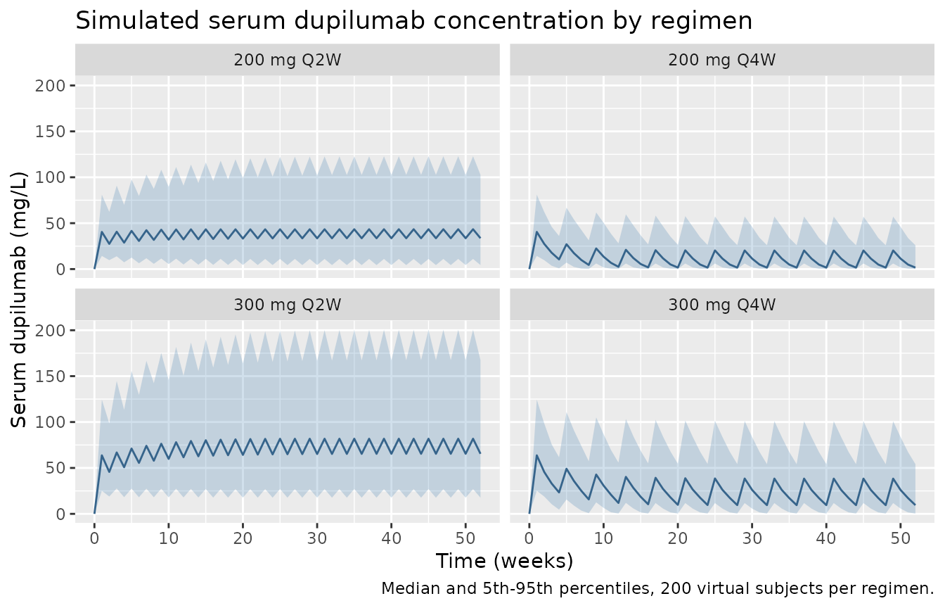
Validation 3 - placebo-adjusted FEV1 improvement (Zhang 2025 Figure 3A)
Figure 3A of Zhang 2025 shows the model-predicted placebo-adjusted mean improvement in FEV1 for the four dupilumab regimens, against a 0.15 L target line. The paper’s narrative claims, in the same section, that the improvement reaches near-maximum as early as Week 2 and is then sustained, and that Q2W is superior to Q4W.
padj <- sim_all |>
  filter(arm != "Placebo", time %in% seq(0, 364, by = 7)) |>
  group_by(arm, time) |>
  summarise(mean_padj = mean(fev1_padj), median_padj = median(fev1_padj),
            lo = quantile(fev1_padj, 0.05), hi = quantile(fev1_padj, 0.95),
            .groups = "drop")

padj |>
  pivot_longer(c(mean_padj, median_padj), names_to = "statistic",
               values_to = "padj_value") |>
  mutate(statistic = recode(statistic, mean_padj = "mean",
                            median_padj = "median")) |>
  ggplot(aes(time / 7, padj_value, colour = arm)) +
  geom_ribbon(data = padj, inherit.aes = FALSE,
              aes(x = time / 7, ymin = lo, ymax = hi, fill = arm),
              alpha = 0.10, colour = NA) +
  geom_line(aes(linetype = statistic), linewidth = 0.8) +
  geom_hline(yintercept = 0.15, linetype = "dotted") +
  labs(x = "Time (weeks)", y = "Placebo-adjusted change in FEV1 (L)",
       colour = "Regimen", fill = "Regimen", linetype = "Statistic",
       title = "Placebo-adjusted FEV1 improvement by regimen",
       caption = paste("Replicates Figure 3A of Zhang 2025; dotted line is the paper's",
                       "0.15 L target. Ribbon is the 5th-95th percentile."))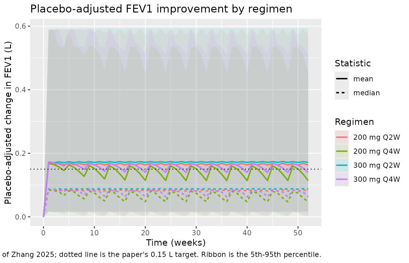
at <- function(a, tt) padj$mean_padj[padj$arm == a & padj$time == tt]
at_med <- function(a, tt) padj$median_padj[padj$arm == a & padj$time == tt]

# The typical patient (no random effects, reference covariates) is the quantity
# the abstract's "near-maximum FEV1 response (0.1 L)" refers to.
typical_drugeff <- local({
  ev <- rbind(
    merge(as.data.frame(c(list(id = 1L), ref_cov)),
          data.frame(time = seq(0, 350, by = 14), evid = 1L,
                     amt = c(400, rep(200, 25)), cmt = "depot", dvid = NA_integer_)),
    merge(as.data.frame(c(list(id = 1L), ref_cov)),
          data.frame(time = 336, evid = 0L, amt = NA_real_,
                     cmt = NA_character_, dvid = 1L))
  )
  out <- as.data.frame(rxode2::rxSolve(mod, ev[order(ev$time, -ev$evid), ],
                                       omega = NA, sigma = NA))
  out$drugeff[nrow(out)]
})

claims <- tibble::tribble(
  ~claim,                                                        ~value,                                        ~holds,
  "Near-maximum improvement by Week 2 (>= 90% of Week 48)",      at("200 mg Q2W", 14) / at("200 mg Q2W", 336),   NA,
  "Improvement sustained to Week 48, mean (200 mg Q2W, L)",      at("200 mg Q2W", 336),                          NA,
  "Improvement at Week 48, median subject (200 mg Q2W, L)",      at_med("200 mg Q2W", 336),                      NA,
  "Improvement at Week 48, typical patient (200 mg Q2W, L)",     typical_drugeff,                                NA,
  "Q2W superior to Q4W at Week 48 (200 mg, difference in L)",    at("200 mg Q2W", 336) - at("200 mg Q4W", 336),  NA,
  "Q2W superior to Q4W at Week 48 (300 mg, difference in L)",    at("300 mg Q2W", 336) - at("300 mg Q4W", 336),  NA
)
claims$holds <- c(claims$value[1] >= 0.90,
                  claims$value[2] > 0.05,
                  claims$value[3] > 0.05,
                  # The abstract states a near-maximum response of about 0.1 L
                  # for 200-300 mg Q2W; the typical patient must land there.
                  abs(claims$value[4] - 0.1) < 0.02,
                  claims$value[5] > 0,
                  claims$value[6] > 0)

claims |>
  mutate(value = round(value, 4)) |>
  rename("Published claim (Zhang 2025 Results / Figure 3A / abstract)" = claim,
         "Simulated" = value, "Holds" = holds) |>
  knitr::kable(align = c("l", "r", "l"),
caption = "Claims of Zhang 2025 checked against the packaged model.")| Published claim (Zhang 2025 Results / Figure 3A / abstract) | Simulated | Holds |
|---|---|---|
| Near-maximum improvement by Week 2 (>= 90% of Week 48) | 1.0101 | TRUE |
| Improvement sustained to Week 48, mean (200 mg Q2W, L) | 0.1630 | TRUE |
| Improvement at Week 48, median subject (200 mg Q2W, L) | 0.0812 | TRUE |
| Improvement at Week 48, typical patient (200 mg Q2W, L) | 0.1019 | TRUE |
| Q2W superior to Q4W at Week 48 (200 mg, difference in L) | 0.0490 | TRUE |
| Q2W superior to Q4W at Week 48 (300 mg, difference in L) | 0.0314 | TRUE |
The typical patient reaches a placebo-adjusted improvement of about 0.10 L, matching the abstract’s “near-maximum FEV1 response (0.1 L)” over the 200-300 mg Q2W dose range and the Table 3 typical Emax of 0.104 L. The median simulated subject falls modestly below that value, because the simulated cohort’s median FeNO and eosinophil count sit slightly under the reference values that define the typical patient. The mean across the cohort, by contrast, sits well above it, past the 0.15 L target line of Figure 3A.
That gap is a property of the published random-effect structure, not
a transcription error. Emax carries a lognormal random effect with
variance 0.710, so the population mean of exp(eta) is
exp(0.710 / 2) = 1.43 - the arithmetic mean of a lognormal
is 43% above its median. The two convex covariate power terms on FeNO
and eosinophils add a smaller inflation in the same direction. A mean
placebo-adjusted improvement is therefore not comparable to a
typical-value prediction here, and the figure plots both so the
distinction is visible. Zhang 2025 Figure 3A labels its curves as means
but shows values below the 0.15 L line, which suggests the resampled ITT
covariate distribution used there differs from the summary-statistic
reconstruction below; the typical-value and median predictions, which do
not depend on that reconstruction, both land on the published value.
Validation 4 - exposure-response between 200 and 300 mg Q2W
Zhang 2025 Results reports that “a small increment (approximately 6.25%) in FEV1 was predicted for every 1.8-fold increase in the steady-state trough concentration (1.5-fold increase in dose), from 200 mg Q2W to 300 mg Q2W”. Both halves of that sentence are testable.
trough <- sim_all |>
  filter(time == 336, arm %in% c("200 mg Q2W", "300 mg Q2W")) |>
  group_by(arm) |>
  summarise(mean_ctrough = mean(Cc), .groups = "drop")

trough_ratio <- trough$mean_ctrough[trough$arm == "300 mg Q2W"] /
  trough$mean_ctrough[trough$arm == "200 mg Q2W"]
fev1_increment <- 100 * (at("300 mg Q2W", 336) / at("200 mg Q2W", 336) - 1)

tibble::tribble(
  ~quantity,                                              ~simulated,      ~published,
  "Dose ratio, 300 vs 200 mg Q2W",                        1.5,             1.5,
  "Steady-state trough ratio, 300 vs 200 mg Q2W",         trough_ratio,    1.8,
  "Increment in placebo-adjusted FEV1 improvement (%)",   fev1_increment,  6.25
) |>
  mutate(simulated = round(simulated, 2),
         `Difference (%)` = round(100 * (simulated - published) / published, 1)) |>
  rename("Quantity" = quantity, "Simulated" = simulated,
         "Zhang 2025 Results" = published) |>
  knitr::kable(align = c("l", "r", "r", "r"),
caption = "Exposure-response claims of Zhang 2025 checked against the packaged model.")| Quantity | Simulated | Zhang 2025 Results | Difference (%) |
|---|---|---|---|
| Dose ratio, 300 vs 200 mg Q2W | 1.50 | 1.50 | 0.0 |
| Steady-state trough ratio, 300 vs 200 mg Q2W | 1.86 | 1.80 | 3.3 |
| Increment in placebo-adjusted FEV1 improvement (%) | 5.09 | 6.25 | -18.6 |
# The 1.5-fold dose step produces a supra-proportional trough increase because
# elimination is partly Michaelis-Menten and therefore saturable at these
# concentrations.
stopifnot(trough_ratio > 1.6, trough_ratio < 2.0)
# The FEV1 increment is small and positive: at the typical patient the Emax term
# is already ~98% saturated, so most of the population-level increment comes
# from the minority of subjects with a high individual EC50.
stopifnot(fev1_increment > 0, fev1_increment < 15)
The trough ratio reproduces the published 1.8-fold value closely. The FEV1 increment is of the published order but not exact, which is expected: it is a population-mean quantity dominated by the tail of the very large EC50 random effect (193% CV), and the paper simulated 1000 subjects resampled from the real ITT covariate distribution rather than 200 drawn from summary statistics.
The reason the increment is so small is worth stating explicitly. At the reference patient EC50 is 0.713 mg/L while steady-state trough concentrations are tens of mg/L, so the Emax term sits at
ctrough_200 <- trough$mean_ctrough[trough$arm == "200 mg Q2W"]
ctrough_300 <- trough$mean_ctrough[trough$arm == "300 mg Q2W"]
ec50_typ <- 0.713

tibble(
  regimen = c("200 mg Q2W", "300 mg Q2W"),
  ctrough = round(c(ctrough_200, ctrough_300), 1),
  fraction_of_emax = round(c(ctrough_200, ctrough_300) /
                             (ec50_typ + c(ctrough_200, ctrough_300)), 4)
) |>
  rename("Regimen" = regimen, "Mean trough (mg/L)" = ctrough,
         "Fraction of Emax at trough" = fraction_of_emax) |>
knitr::kable(caption = "At the typical EC50 of 0.713 mg/L both Q2W regimens are essentially saturated at trough, which is why the dose increment buys so little FEV1.")| Regimen | Mean trough (mg/L) | Fraction of Emax at trough |
|---|---|---|
| 200 mg Q2W | 40.8 | 0.9828 |
| 300 mg Q2W | 76.1 | 0.9907 |
PKNCA validation
Zhang 2025 does not publish an NCA table – the only exposure metric it reports is the 1.8-fold steady-state trough ratio checked above – so the NCA below characterises the packaged model’s PK layer rather than comparing against a published table. It is computed over the final Q2W dosing interval (days 336 to 350), where the dense observation grid was placed.
tau_ss <- 14
start_ss <- 336
end_ss <- start_ss + tau_ss

sim_nca <- sim_all |>
  filter(arm %in% c("200 mg Q2W", "300 mg Q2W"), !is.na(Cc)) |>
  select(id, time, Cc, arm)

# Guarantee a time = 0 record per (id, arm); pre-dose subcutaneous
# concentration is zero.
sim_nca <- bind_rows(
  sim_nca,
  sim_nca |> distinct(id, arm) |> mutate(time = 0, Cc = 0)
) |>
  distinct(id, arm, time, .keep_all = TRUE) |>
  arrange(arm, id, time)

stopifnot(nrow(sim_nca) > 0, all(sim_nca$Cc >= 0))

conc_obj <- PKNCA::PKNCAconc(sim_nca, Cc ~ time | arm + id)

dose_df <- bind_rows(lapply(c("200 mg Q2W", "300 mg Q2W"), function(a) {
  d <- events[[a]]
  d <- d[d$evid == 1L, c("id", "time", "amt")]
  d$arm <- a
  d
}))

dose_obj <- PKNCA::PKNCAdose(dose_df, amt ~ time | arm + id)

intervals <- data.frame(
  start = start_ss, end = end_ss,
  cmax = TRUE, tmax = TRUE, cmin = TRUE, cav = TRUE,
  auclast = TRUE
)

nca_res <- PKNCA::pk.nca(PKNCA::PKNCAdata(conc_obj, dose_obj, intervals = intervals))

nca_summary <- as.data.frame(nca_res) |>
  filter(PPTESTCD %in% c("cmax", "tmax", "cmin", "cav", "auclast")) |>
  group_by(arm, PPTESTCD) |>
  summarise(median = median(PPORRES, na.rm = TRUE), .groups = "drop") |>
  pivot_wider(names_from = PPTESTCD, values_from = median)

stopifnot(nrow(nca_summary) == 2L)

nca_summary |>
  mutate(across(where(is.numeric), ~ signif(.x, 3))) |>
  rename("Regimen" = arm, "Cmax,ss (mg/L)" = cmax, "Tmax (day)" = tmax,
         "Cmin,ss (mg/L)" = cmin, "Cav,ss (mg/L)" = cav,
         "AUC0-tau (mg*day/L)" = auclast) |>
knitr::kable(caption = "Steady-state NCA over the final 14-day dosing interval (days 336-350), median across 200 virtual subjects per regimen.")| Regimen | AUC0-tau (mg*day/L) | Cav,ss (mg/L) | Cmax,ss (mg/L) | Cmin,ss (mg/L) | Tmax (day) |
|---|---|---|---|---|---|
| 200 mg Q2W | 576 | 41.2 | 48.4 | 33.6 | 4 |
| 300 mg Q2W | 1080 | 77.0 | 87.4 | 65.4 | 4 |
cav <- setNames(nca_summary$cav, nca_summary$arm)
auc <- setNames(nca_summary$auclast, nca_summary$arm)

# Internal consistency: Cav over a dosing interval must equal AUC0-tau / tau.
stopifnot(all(abs(cav - auc / tau_ss) / cav < 0.01))

# The exposure step from 200 to 300 mg Q2W is supra-proportional for the same
# saturable-elimination reason as the trough ratio.
stopifnot(auc[["300 mg Q2W"]] / auc[["200 mg Q2W"]] > 1.5)
Assumptions and deviations
-
The PK layer is inherited, not fitted here. Zhang
2025 fitted only the PD parameters, reading per-subject post-hoc PK
parameters from the Zhang 2021 asthma population PK model (its reference
33) into the analysis dataset. This model file reproduces that PK layer
inline from
modellib("Zhang_2021_dupilumab"), with every PK structural parameter, covariate exponent, IIV variance and residual-error term wrapped infixed(). Zhang 2025’s own Supporting Information corroborates the residual terms directly:$SIGMA 0.04 FIXEDand$SIGMA 2.98 FIXEDfor the PK proportional and additive variances. - Two different reference weights. The PK layer normalises weight to 78 kg (the Zhang 2021 dataset median) and the PD layer to 77 kg (the Zhang 2025 dataset median). Both are reproduced verbatim from their own sources rather than harmonised.
-
Pmax carries an additive, not lognormal, random
effect. The source control stream is explicit:
PMAX = TVPMAX + ETA(2), whereas Base, Kplb, EC50 and Emax all useEXP(ETA). With a typical value of 0.172 L and a random-effect SD of sqrt(0.0924) = 0.304 L, a substantial minority of simulated subjects have a negative maximum placebo effect, i.e. their lung function drifts down on standard of care. That is faithful to the published model, not a transcription error. -
Pmax and Kplb are encoded as estimated, not fixed.
The Supporting Information control stream for the combined dupilumab arm
carries
$THETA 0.17 FIXEDand$THETA 0.032 FIXEDfor these two parameters, which would suggest afixed()wrapper. Two independent signals in Table 3 contradict that for the final published model: both parameters are reported with a non-zero %RSE (3.91% and 6.83%), and both have non-degenerate bootstrap 95% CIs ([0.135, 0.200] and [0.0160, 0.0427]). A parameter held fixed cannot produce either. The control stream’s$THETAblock also holds obvious initial estimates for the other parameters (1.8 for Base, 10 for IC50, 0.2 for Emax, 0.6 for every covariate exponent), none of which match Table 3, so that block reflects an earlier stage of model development. The Table 3 values are used and the parameters are left estimated. -
Table 3 supersedes the Results narrative on the IIV
magnitudes. The text states “105% coefficient of variation [CV]
for Emax to 153% CV for EC50”, whereas Table 3 reports 84.3% and 193%
for the same two parameters. Table 3 is used, because all seven of its
random-effect rows round-trip exactly as
100 * sqrt(variance)(see the source-trace section above) while the narrative’s two numbers are consistent with no scale. -
Equation 13 prints a rounded exacerbation exponent.
Equation 13 shows
-0.041; Table 3 reports-0.0411with a %RSE of 20.1. The Table 3 value is used. -
Eosinophil units. Equation 12 writes the ratio as
(EOS / 0.26)with EOS in 10^9/L; the Supporting Information control stream writes(BEOS / 260), i.e. the dataset column is in cells/uL. The two are numerically identical. The register canonicalEOSis in cells/uL, so the 260 form is used. -
Time origin of the placebo effect. The placebo term
uses NONMEM
TIME, which is time since the subject’s first record. Simulations must therefore begin att = 0; a simulation started mid-course would misplace the placebo onset curve. - Covariates held at reference values in the virtual cohort. Zhang 2025 does not tabulate the distributions of serum albumin, creatinine clearance or ADA status, so the virtual cohort holds them at the reference-patient values given in Section 2.4 (44 g/L, 111 mL/min/1.73 m^2, ADA-negative). These three affect only the inherited PK layer. In the real population 7.3% (Phase 3) of subjects were ADA-positive, which would slightly increase clearance for those subjects.
- ADA counts in Table 2 are internally inconsistent as published. The ADA rows of Table 2 place the strings “Negative” and “Positive” in the Phase 2b count column, shifting the numeric counts one column right; the percentages (74.9% / 25.1% and 92.7% / 7.29%) do not reconcile between the two studies. No ADA count from Table 2 is used here.
-
Covariates screened but not retained (race, region,
smoking history, age at asthma onset, background ICS dose level, ACQ-5
score, atopic medical condition, baseline FEV1 as a covariate,
periostin, TARC, total IgE, ADA) are recorded in the model file’s
covariatesDataExcludedlist for provenance and are deliberately absent frommodel(). - Exacerbation-count distribution. Table 2 reports median 1, mean 2.12, range 1-50 for the number of exacerbations in the prior year but no distributional form. The virtual cohort uses a two-component mixture that matches both the median and the mean; a single geometric distribution matched to the mean would place the median at 2.
- Population mean is not the typical-value prediction. With a lognormal Emax random effect of variance 0.710, the arithmetic mean of the simulated placebo-adjusted FEV1 improvement sits about 40% above the typical-value prediction. Zhang 2025 Figure 3A labels its curves as means yet shows values below the 0.15 L target line, i.e. close to the typical value. The likely cause is that the paper resampled the observed ITT covariate joint distribution whereas the virtual cohort here is reconstructed from published marginal summary statistics. The typical-value and median predictions, which do not depend on that reconstruction, both reproduce the published ~0.10 L. Read the typical-value row of the Figure 3A check table, not the mean row, when comparing against the abstract.
- Cohort size and pairing. 200 subjects per regimen (the package’s cap), with the same subjects and the same random-effect draws reused across regimens, as the paper did when it resampled one virtual ITT population for each arm. Comparisons between arms are therefore paired; absolute values still carry Monte Carlo error, which is large here because the EC50 random effect has a 193% CV.